7.10 Extracting values from stars for vector data
7.10.1 Points
We can extract the value of raster cells in which points are located (exactly like Chapter 5) using st_extract().
Let’s first create points data that are randomly located inside Michigan.
Here is what the generated points look like:
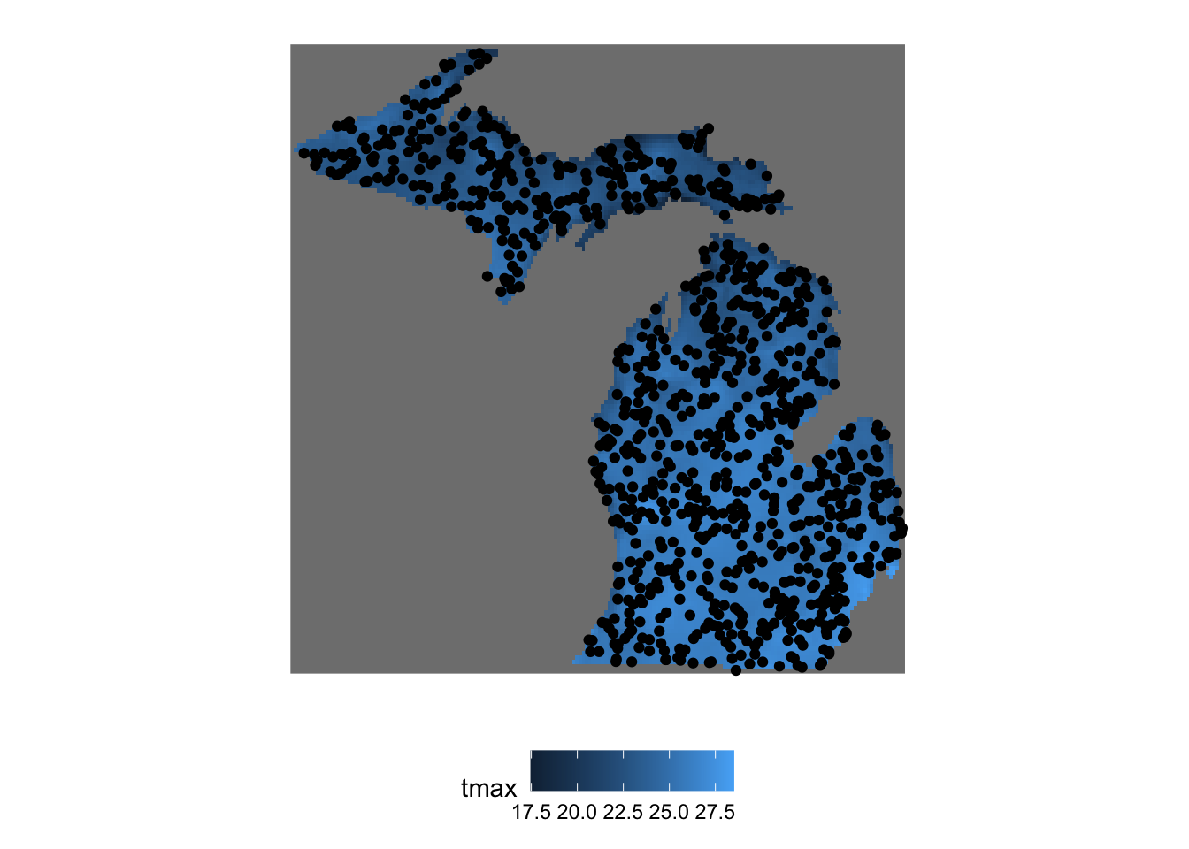
Figure 7.8: Map of randomly located points inside Michigan
We now extract the value of rasters in which points are located:
Simple feature collection with 1000 features and 10 fields
geometry type:  POINT
dimension:      XY
bbox:           xmin: -90.26031 ymin: 41.71712 xmax: -82.47312 ymax: 47.43735
geographic CRS: NAD83
First 10 features:
   2009-01-01 2009-01-02 2009-01-03 2009-01-04 2009-01-05 2009-01-06 2009-01-07
1      25.450     25.727     24.810     27.087     29.131     22.974     25.247
2      21.029     18.575     20.100     21.445     18.854     19.699     20.109
3      21.757     22.835     21.778     22.979     21.894     21.873     22.121
4      23.637     26.514     24.561     25.808     29.675     22.183     23.904
5      22.868     19.672     20.685     23.881     20.625     21.422     21.553
6      24.280     22.298     21.853     23.678     22.827     22.326     23.254
7      22.751     19.308     20.950     22.155     20.325     20.560     21.333
8      24.793     25.775     24.474     26.520     28.726     23.518     24.486
9      25.878     26.348     23.853     27.044     28.963     24.661     25.572
10     24.918     21.120     22.429     25.840     22.183     22.865     23.427
   2009-01-08 2009-01-09 2009-01-10                        sfc
1      23.726     23.338     32.184 POINT (-83.34935 43.49406)
2      20.965     22.658     22.536 POINT (-88.20274 46.66783)
3      20.369     19.555     29.512 POINT (-83.50303 45.32732)
4      21.052     22.764     32.978 POINT (-82.47312 43.03622)
5      20.193     26.205     25.094 POINT (-89.91415 46.33971)
6      21.973     22.260     28.648 POINT (-84.57265 44.56324)
7      23.214     22.396     23.083 POINT (-88.43553 47.33342)
8      23.078     23.250     32.018    POINT (-83.014 43.4846)
9      25.717     25.521     32.768 POINT (-84.04252 42.82157)
10     21.740     24.730     27.868 POINT (-87.85009 46.39967)
As you can see each date forms a column of extracted values for the points because the third dimension of tmax_MI is Dates object. So, you can easily turn the outcome to an sf object with date as Date object as follows.
pivot_longer(extracted_tmax, - sfc, names_to = "date", values_to = "tmax") %>%
  st_as_sf() %>%
  mutate(date = ymd(date))
Simple feature collection with 10000 features and 2 fields
geometry type: POINT
dimension: XY
bbox: xmin: -90.26031 ymin: 41.71712 xmax: -82.47312 ymax: 47.43735
geographic CRS: NAD83
# A tibble: 10,000 x 3
sfc date tmax
* <POINT [°]> <date> <dbl>
1 (-83.34935 43.49406) 2009-01-01 25.5
2 (-83.34935 43.49406) 2009-01-02 25.7
3 (-83.34935 43.49406) 2009-01-03 24.8
4 (-83.34935 43.49406) 2009-01-04 27.1
5 (-83.34935 43.49406) 2009-01-05 29.1
6 (-83.34935 43.49406) 2009-01-06 23.0
7 (-83.34935 43.49406) 2009-01-07 25.2
8 (-83.34935 43.49406) 2009-01-08 23.7
9 (-83.34935 43.49406) 2009-01-09 23.3
10 (-83.34935 43.49406) 2009-01-10 32.2
# … with 9,990 more rowsYou cannot extract values from multiple attributes at the same time.
Error in sf::gdal_write(obj, ..., file = dsn, driver = driver, options = options, : dimensions don't matchaggregate() is much slower compared to terra::extract(), which is discussed in section 5. So, if you are finding the speed of extraction an issue, you can do the following:
- convert the
starsobject to aSpatRasterobject - use terra::extract() to extract values for the vector data
- assign the date values to the
data.frameof extracted values
#--- Step 1: stars to RasterBrick to SpatRaster ---#
tmax_MI_sr <- tmax_MI %>%
  #--- to RasterBrick ---#
  as("Raster") %>%
  #--- to SpatRaster ---#
  rast()

#--- Step 2: extraction ---#
extracted_values <- terra::extract(tmax_MI_sr, st_coordinates(MI_points)) %>%
  data.frame() %>%
  #--- assign id ---#
  mutate(id = MI_points$id)

#--- Step 3: assign dates as the variable names ---#
date_values <- as.character(st_get_dimension_values(tmax_MI, "date"))
names(extracted_values) <- c(date_values, "id")

#--- wide to long ---#
pivot_longer(extracted_values, -id, , names_to = "date", values_to = "tmax")
I must say, this is quite a hassle in terms of coding. But, if you need to do extraction jobs fast many many times, this approach may be beneficial.
7.10.2 Polygons
In order to extract cell values from stars objects (just like Chapter 5) and summarize them for polygons, you can aggregate().
Let’s create polygons such that they cover Michigan:
Here is what it looks like (Figure 7.9):
ggplot() +
  geom_stars(data = tmax_MI[,,,1]) +
  geom_sf(data = MI_polygons, fill = NA) +
  theme_for_map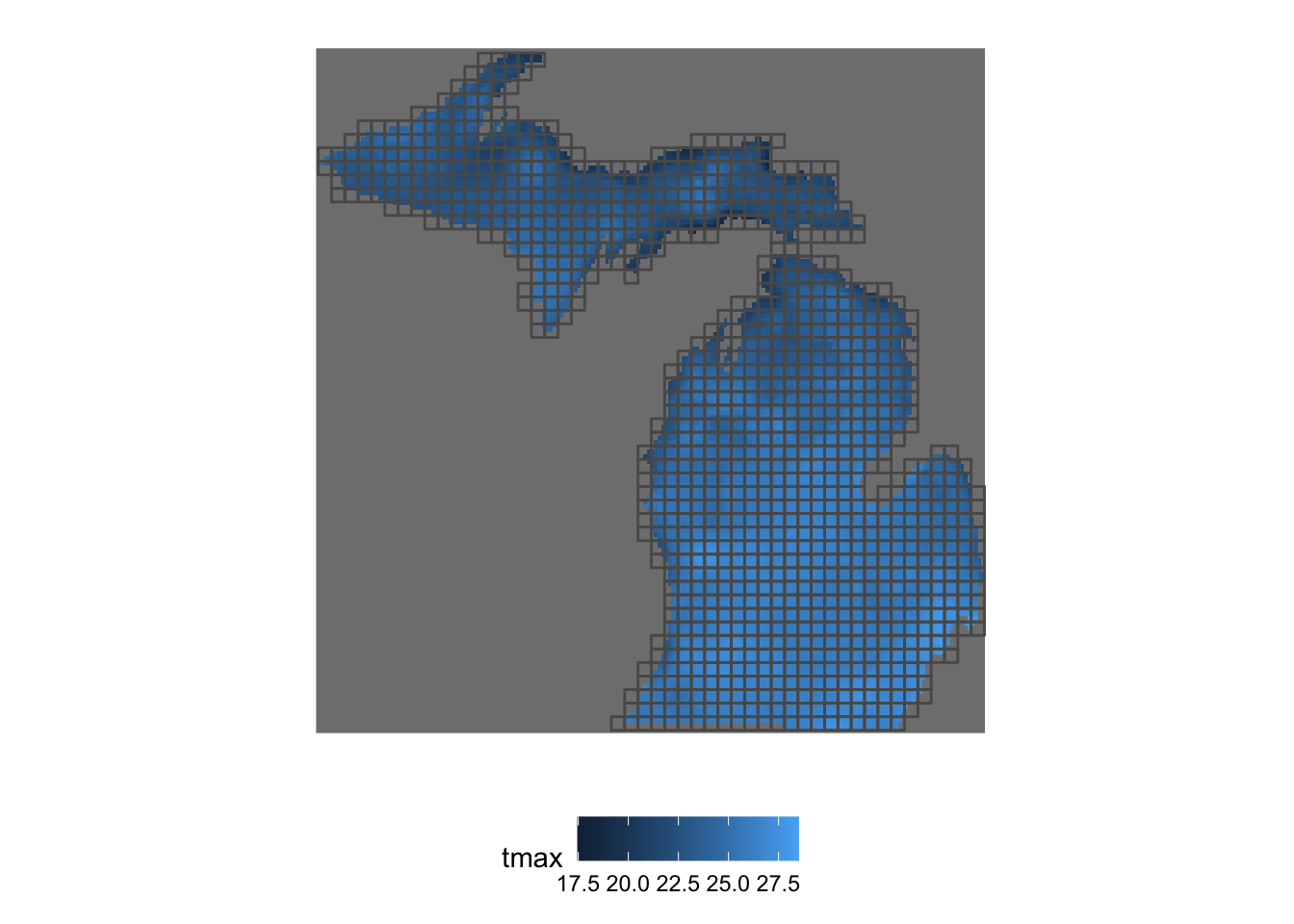
Figure 7.9: Map of regularly-sized polygons over Michigan
For example this will find the mean of the tmax values for each polygon:
Simple feature collection with 1064 features and 10 fields
geometry type:  POLYGON
dimension:      XY
bbox:           xmin: -90.41273 ymin: 41.71133 xmax: -82.44289 ymax: 47.48101
geographic CRS: NAD83
First 10 features:
   2009-01-01 2009-01-02 2009-01-03 2009-01-04 2009-01-05 2009-01-06 2009-01-07
1          NA         NA         NA         NA         NA         NA         NA
2          NA         NA         NA         NA         NA         NA         NA
3          NA         NA         NA         NA         NA         NA         NA
4          NA         NA         NA         NA         NA         NA         NA
5          NA         NA         NA         NA         NA         NA         NA
6          NA         NA         NA         NA         NA         NA         NA
7          NA         NA         NA         NA         NA         NA         NA
8          NA         NA         NA         NA         NA         NA         NA
9          NA         NA         NA         NA         NA         NA         NA
10         NA         NA         NA         NA         NA         NA         NA
   2009-01-08 2009-01-09 2009-01-10                              x
1          NA         NA         NA POLYGON ((-86.906 41.71133,...
2          NA         NA         NA POLYGON ((-86.74661 41.7113...
3          NA         NA         NA POLYGON ((-86.58721 41.7113...
4          NA         NA         NA POLYGON ((-86.42781 41.7113...
5          NA         NA         NA POLYGON ((-86.26842 41.7113...
6          NA         NA         NA POLYGON ((-86.10902 41.7113...
7          NA         NA         NA POLYGON ((-85.94962 41.7113...
8          NA         NA         NA POLYGON ((-85.79023 41.7113...
9          NA         NA         NA POLYGON ((-85.63083 41.7113...
10         NA         NA         NA POLYGON ((-85.47143 41.7113...
Oops, so many NAs! This is clearly because many polygons intersect with cells that have NA values. To avoid this, we can add na.rm=TRUE option like this:
Simple feature collection with 1064 features and 10 fields
geometry type:  POLYGON
dimension:      XY
bbox:           xmin: -90.41273 ymin: 41.71133 xmax: -82.44289 ymax: 47.48101
geographic CRS: NAD83
First 10 features:
   2009-01-01 2009-01-02 2009-01-03 2009-01-04 2009-01-05 2009-01-06 2009-01-07
1    26.65600   23.98400   23.89500   28.33900   26.07500   23.85000   24.39900
2    26.04367   24.34467   23.89733   28.45467   26.54600   24.28400   24.56967
3    25.73825   24.87400   23.97600   28.76300   27.26975   25.34700   25.27225
4    25.87100   25.17925   24.11325   29.06600   27.85700   25.98200   25.78500
5    25.70775   25.48625   24.11050   28.94025   27.95825   26.21000   25.90000
6    25.57850   25.64950   24.14375   28.74075   28.05550   26.18900   25.85250
7    25.78925   25.75600   24.19150   28.65325   28.15450   26.45800   26.12075
8    26.04167   25.81667   24.33033   28.58833   28.35567   26.91667   26.40033
9    26.04475   26.06450   24.21250   28.53550   28.27700   26.67875   26.60900
10   26.14425   26.46525   24.13775   28.64750   28.56825   26.36500   26.83575
   2009-01-08 2009-01-09 2009-01-10                              x
1    22.35300   30.46500   31.82900 POLYGON ((-86.906 41.71133,...
2    22.76133   30.39567   31.98000 POLYGON ((-86.74661 41.7113...
3    23.05250   30.66375   32.50500 POLYGON ((-86.58721 41.7113...
4    23.27725   30.97350   33.02000 POLYGON ((-86.42781 41.7113...
5    23.70050   30.78825   33.31025 POLYGON ((-86.26842 41.7113...
6    24.21475   30.35250   33.41150 POLYGON ((-86.10902 41.7113...
7    24.51575   30.16125   33.44150 POLYGON ((-85.94962 41.7113...
8    24.67367   30.01033   33.43500 POLYGON ((-85.79023 41.7113...
9    25.00725   30.10925   33.43200 POLYGON ((-85.63083 41.7113...
10   25.59000   30.30200   33.72700 POLYGON ((-85.47143 41.7113...
Note that this would not work:
Error in mean.default(na.rm = TRUE): argument "x" is missing, with no defaultwhich is the first thing I tried before I googled the problem.
Right now, the aggregate() function is slower for large raster data than exact_extract(), which we saw in Chapter 5. If the extraction speed of aggregate() is not satisfactory for your applications, you could just convert the stars object to RasterBrick using the as() method (section 7.8) and then use exact_extract() as follows:
The good news is, exact_extract() is coming soon to the aggregate() methods for stars (see here), which means that you do not have to do these tedious conversions. Actually, if you are willing to install the version in development, you can add exact = TRUE option to take advantage of the speed of exact_extract().