3.3 Spatial Join
By spatial join, we mean spatial operations that involve all of the following:
- overlay one spatial layer (target layer) onto another spatial layer (source layer)
- for each of the observation in the target layer
- identify which objects in the source layer it geographically intersects (or a different topological relation) with
- extract values associated with the intersecting objects in the source layer (and summarize if necessary),
- assign the extracted value to the object in the target layer
- identify which objects in the source layer it geographically intersects (or a different topological relation) with
For economists, this is probably the most common motivation for using GIS software, with the ultimate goal being to include the spatially joined variables as covariates in regression analysis.
We can classify spatial join into four categories by the type of the underlying spatial objects:
- vector-vector: vector data (target) against vector data (source)
- vector-raster: vector data (target) against raster data (source)
- raster-vector: raster data (target) against vector data (source)
- raster-raster: raster data (target) against raster data (source)
Among the four, our focus here is the first case. The second case will be discussed in Chapter 5. We will not cover the third and fourth cases in this course because it is almost always the case that our target data is a vector data (e.g., city or farm fields as points, political boundaries as polygons, etc).
Category 1 can be further broken down into different sub categories depending on the type of spatial object (point, line, and polygon). Here, we will ignore any spatial joins that involve lines. This is because objects represented by lines are rarely observation units in econometric analysis nor the source data from which we will extract values.60 Here is the list of the types of spatial joins we will learn.
- points (target) against polygons (source)
- polygons (target) against points (source)
- polygons (target) against polygons (source)
3.3.1 Case 1: points (target) vs polygons (source)
Case 1, for each of the observations (points) in the target data, finds which polygon in the source data it intersects, and then assign the value associated with the polygon to the point61. In order to achieve this, we can use the st_join() function, whose syntax is as follows:
#--- this does not run ---#
st_join(target_sf, source_sf)
Similar to spatial subsetting, the default topological relation is st_intersects()62.
We use the Kansas irrigation well data (points) and Kansas county boundary data (polygons) for a demonstration. Our goal is to assign the county-level corn price information from the Kansas county data to wells. First let me create and add a fake county-level corn price variable to the Kansas county data.
KS_corn_price <- KS_counties %>%
  mutate(corn_price = seq(3.2, 3.9, length = nrow(.))) %>%
  dplyr::select(COUNTYFP, corn_price)
Here is the map of Kansas counties color-differentiated by fake corn price (Figure 3.16):
tm_shape(KS_corn_price) +
  tm_polygons(col = "corn_price") +
  tm_layout(frame = FALSE, legend.outside = TRUE)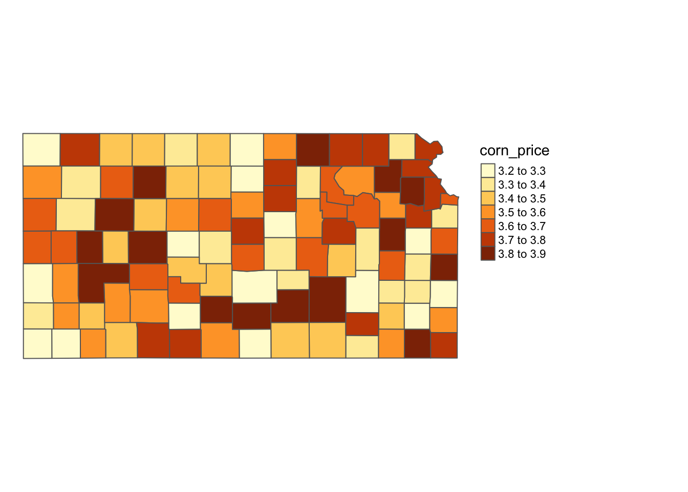
Figure 3.16: Map of county-level fake corn price
For this particular context, the following code will do the job:
#--- spatial join ---#
(
KS_wells_County <- st_join(KS_wells, KS_corn_price)
)
Simple feature collection with 37647 features and 5 fields
Geometry type: POINT
Dimension: XY
Bounding box: xmin: -102.0495 ymin: 36.99552 xmax: -94.62089 ymax: 40.00199
Geodetic CRS: NAD83
First 10 features:
site af_used in_hpa COUNTYFP corn_price geometry
1 1 232.099948 TRUE 069 3.556731 POINT (-100.4423 37.52046)
2 3 13.183940 TRUE 039 3.449038 POINT (-100.7118 39.91526)
3 5 99.187052 TRUE 165 3.287500 POINT (-99.15168 38.48849)
4 7 0.000000 TRUE 199 3.644231 POINT (-101.8995 38.78077)
5 8 145.520499 TRUE 055 3.832692 POINT (-100.7122 38.0731)
6 9 3.614535 FALSE 143 3.799038 POINT (-97.70265 39.04055)
7 11 188.423543 TRUE 181 3.590385 POINT (-101.7114 39.55035)
8 12 77.335960 FALSE 177 3.550000 POINT (-95.97031 39.16121)
9 15 0.000000 TRUE 159 3.610577 POINT (-98.30759 38.26787)
10 17 167.819034 TRUE 069 3.556731 POINT (-100.2785 37.71539)You can see from Figure 3.17 below that all the wells inside the same county have the same corn price value.
tm_shape(KS_counties) +
  tm_polygons() +
tm_shape(KS_wells_County) +
  tm_symbols(col = "corn_price", size = 0.1) +
  tm_layout(frame = FALSE, legend.outside = TRUE)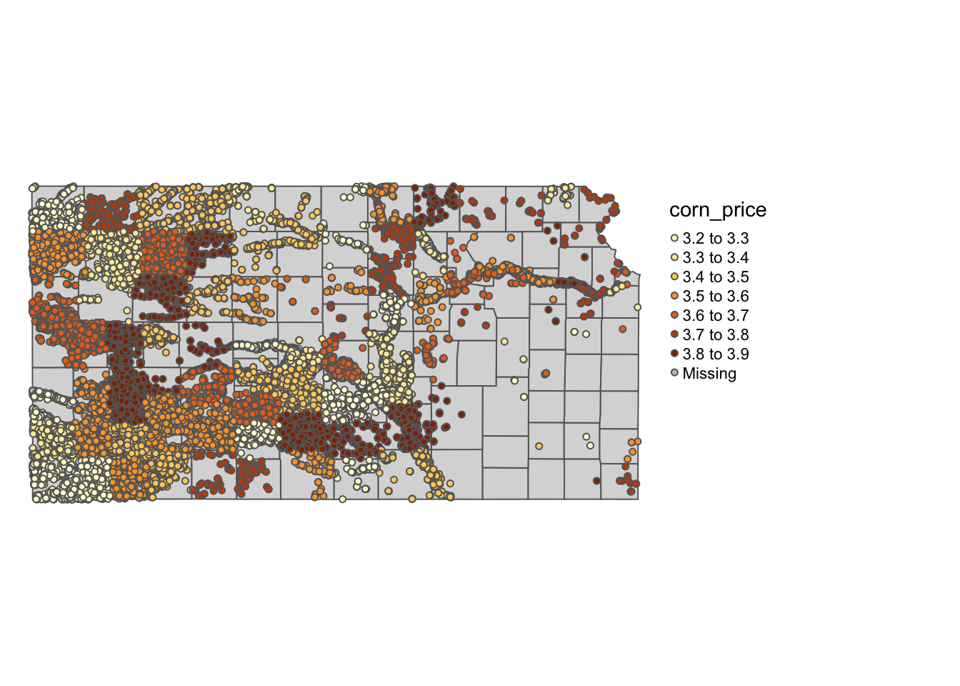
Figure 3.17: Map of wells color-differentiated by corn price
3.3.2 Case 2: polygons (target) vs points (source)
Case 2, for each of the observations (polygons) in the target data, find which observations (points) in the source data it intersects, and then assign the values associated with the points to the polygon. We use the same function: st_join()63.
Suppose you are now interested in county-level analysis and you would like to get county-level total groundwater pumping. The target data is KS_counties, and the source data is KS_wells.
#--- spatial join ---#
KS_County_wells <- st_join(KS_counties, KS_wells)

#--- take a look ---#
dplyr::select(KS_County_wells, COUNTYFP, site, af_used)
Simple feature collection with 37652 features and 3 fields
Geometry type: MULTIPOLYGON
Dimension: XY
Bounding box: xmin: -102.0517 ymin: 36.99308 xmax: -94.59193 ymax: 40.00308
Geodetic CRS: NAD83
First 10 features:
COUNTYFP site af_used geometry
1 133 53861 17.01790 MULTIPOLYGON (((-95.5255 37...
1.1 133 70592 0.00000 MULTIPOLYGON (((-95.5255 37...
2 075 328 394.04513 MULTIPOLYGON (((-102.0446 3...
2.1 075 336 80.65036 MULTIPOLYGON (((-102.0446 3...
2.2 075 436 568.25359 MULTIPOLYGON (((-102.0446 3...
2.3 075 1007 215.80416 MULTIPOLYGON (((-102.0446 3...
2.4 075 1170 0.00000 MULTIPOLYGON (((-102.0446 3...
2.5 075 1192 77.39120 MULTIPOLYGON (((-102.0446 3...
2.6 075 1249 0.00000 MULTIPOLYGON (((-102.0446 3...
2.7 075 1300 320.22612 MULTIPOLYGON (((-102.0446 3...As you can see in the resulting dataset, all the unique polygon - point intersecting combinations comprise the observations. For each of the polygons, you will have as many observations as the number of wells that intersect with the polygon. Once you join the two layers, you can find statistics by polygon (county here). Since we want groundwater extraction by county, the following does the job.
KS_County_wells %>%
  group_by(COUNTYFP) %>%
  summarize(af_used = sum(af_used, na.rm = TRUE))
Simple feature collection with 105 features and 2 fields
Geometry type: POLYGON
Dimension: XY
Bounding box: xmin: -102.0517 ymin: 36.99308 xmax: -94.59193 ymax: 40.00308
Geodetic CRS: NAD83
# A tibble: 105 × 3
COUNTYFP af_used geometry
<fct> <dbl> <POLYGON [°]>
1 001 0 ((-95.5255 37.73276, -95.08808 37.73248, -95.07969 37.8198,…
2 003 0 ((-95.51897 38.03823, -95.07788 38.03771, -95.06583 38.3899…
3 005 771. ((-95.57035 39.41905, -95.18089 39.41922, -94.99785 39.4188…
4 007 4972. ((-99.0115 37.38426, -99.00138 37.37502, -99.0003 36.99936,…
5 009 61083. ((-99.03241 38.34833, -99.03231 38.26123, -98.91258 38.2610…
6 011 0 ((-95.08801 37.67452, -94.61787 37.67311, -94.61789 37.6822…
7 013 480. ((-95.78894 39.653, -95.56413 39.65287, -95.33974 39.65298,…
8 015 343. ((-97.15333 37.47554, -96.52569 37.4764, -96.5253 37.60701,…
9 017 0 ((-96.84077 38.08562, -96.52278 38.08637, -96.3581 38.08582…
10 019 0 ((-96.52558 36.99868, -96.50029 36.99864, -96.21757 36.9990…
# … with 95 more rowsOf course, it is just as easy to get other types of statistics by simply modifying the summarize() part.
However, this two-step process can actually be done in one step using aggregate(), in which you specify how you want to aggregate with the FUN option as follows:
#--- mean ---#
aggregate(KS_wells, KS_counties, FUN = mean)
Simple feature collection with 105 features and 3 fields
Geometry type: MULTIPOLYGON
Dimension: XY
Bounding box: xmin: -102.0517 ymin: 36.99308 xmax: -94.59193 ymax: 40.00308
Geodetic CRS: NAD83
First 10 features:
site af_used in_hpa geometry
1 62226.50 8.508950 0.0000000 MULTIPOLYGON (((-95.5255 37...
2 35153.23 175.890557 0.4466292 MULTIPOLYGON (((-102.0446 3...
3 40086.82 35.465123 0.0000000 MULTIPOLYGON (((-98.48738 3...
4 40191.67 286.324733 1.0000000 MULTIPOLYGON (((-101.5566 3...
5 51256.15 46.013373 0.9743976 MULTIPOLYGON (((-98.47279 3...
6 33033.13 202.612377 1.0000000 MULTIPOLYGON (((-102.0419 3...
7 29840.40 0.000000 0.0000000 MULTIPOLYGON (((-96.52278 3...
8 28235.82 94.585634 0.9736842 MULTIPOLYGON (((-102.0517 4...
9 36180.06 44.033911 0.3000000 MULTIPOLYGON (((-98.50445 4...
10 40016.00 1.142775 0.0000000 MULTIPOLYGON (((-95.50827 3...#--- sum ---#
aggregate(KS_wells, KS_counties, FUN = sum)Simple feature collection with 105 features and 3 fields
Geometry type: MULTIPOLYGON
Dimension: XY
Bounding box: xmin: -102.0517 ymin: 36.99308 xmax: -94.59193 ymax: 40.00308
Geodetic CRS: NAD83
First 10 features:
site af_used in_hpa geometry
1 124453 1.701790e+01 0 MULTIPOLYGON (((-95.5255 37...
2 12514550 6.261704e+04 159 MULTIPOLYGON (((-102.0446 3...
3 1964254 1.737791e+03 0 MULTIPOLYGON (((-98.48738 3...
4 42442400 3.023589e+05 1056 MULTIPOLYGON (((-101.5566 3...
5 68068173 6.110576e+04 1294 MULTIPOLYGON (((-98.47279 3...
6 15756801 9.664610e+04 477 MULTIPOLYGON (((-102.0419 3...
7 149202 0.000000e+00 0 MULTIPOLYGON (((-96.52278 3...
8 17167377 5.750807e+04 592 MULTIPOLYGON (((-102.0517 4...
9 1809003 2.201696e+03 15 MULTIPOLYGON (((-98.50445 4...
10 160064 4.571102e+00 0 MULTIPOLYGON (((-95.50827 3...Notice that the mean() function was applied to all the columns in KS_wells, including site id number. So, you might want to select variables you want to join before you apply the aggregate() function like this:
aggregate(dplyr::select(KS_wells, af_used), KS_counties, FUN = mean)Simple feature collection with 105 features and 1 field
Geometry type: MULTIPOLYGON
Dimension: XY
Bounding box: xmin: -102.0517 ymin: 36.99308 xmax: -94.59193 ymax: 40.00308
Geodetic CRS: NAD83
First 10 features:
af_used geometry
1 8.508950 MULTIPOLYGON (((-95.5255 37...
2 175.890557 MULTIPOLYGON (((-102.0446 3...
3 35.465123 MULTIPOLYGON (((-98.48738 3...
4 286.324733 MULTIPOLYGON (((-101.5566 3...
5 46.013373 MULTIPOLYGON (((-98.47279 3...
6 202.612377 MULTIPOLYGON (((-102.0419 3...
7 0.000000 MULTIPOLYGON (((-96.52278 3...
8 94.585634 MULTIPOLYGON (((-102.0517 4...
9 44.033911 MULTIPOLYGON (((-98.50445 4...
10 1.142775 MULTIPOLYGON (((-95.50827 3...3.3.3 Case 3: polygons (target) vs polygons (source)
For this case, st_join(target_sf, source_sf) will return all the unique intersecting polygon-polygon combinations with the information of the polygon from source_sf attached.
We will use county-level corn acres in Iowa in 2018 from USDA NASS64 and Hydrologic Units65 Our objective here is to find corn acres by HUC units based on the county-level corn acres data66.
We first import the Iowa corn acre data:
#--- IA boundary ---#
IA_corn <- readRDS("Data/IA_corn.rds")

#--- take a look ---#
IA_corn
Simple feature collection with 93 features and 3 fields
Geometry type: MULTIPOLYGON
Dimension: XY
Bounding box: xmin: 203228.6 ymin: 4470941 xmax: 736832.9 ymax: 4822687
Projected CRS: NAD83 / UTM zone 15N
First 10 features:
county_code year acres geometry
1 083 2018 183500 MULTIPOLYGON (((458997 4711...
2 141 2018 167000 MULTIPOLYGON (((267700.8 47...
3 081 2018 184500 MULTIPOLYGON (((421231.2 47...
4 019 2018 189500 MULTIPOLYGON (((575285.6 47...
5 023 2018 165500 MULTIPOLYGON (((497947.5 47...
6 195 2018 111500 MULTIPOLYGON (((459791.6 48...
7 063 2018 110500 MULTIPOLYGON (((345214.3 48...
8 027 2018 183000 MULTIPOLYGON (((327408.5 46...
9 121 2018 70000 MULTIPOLYGON (((396378.1 45...
10 077 2018 107000 MULTIPOLYGON (((355180.1 46...Here is the map of Iowa counties color-differentiated by corn acres (Figure 3.18):
#--- here is the map ---#
tm_shape(IA_corn) +
  tm_polygons(col = "acres") +
  tm_layout(frame = FALSE, legend.outside = TRUE)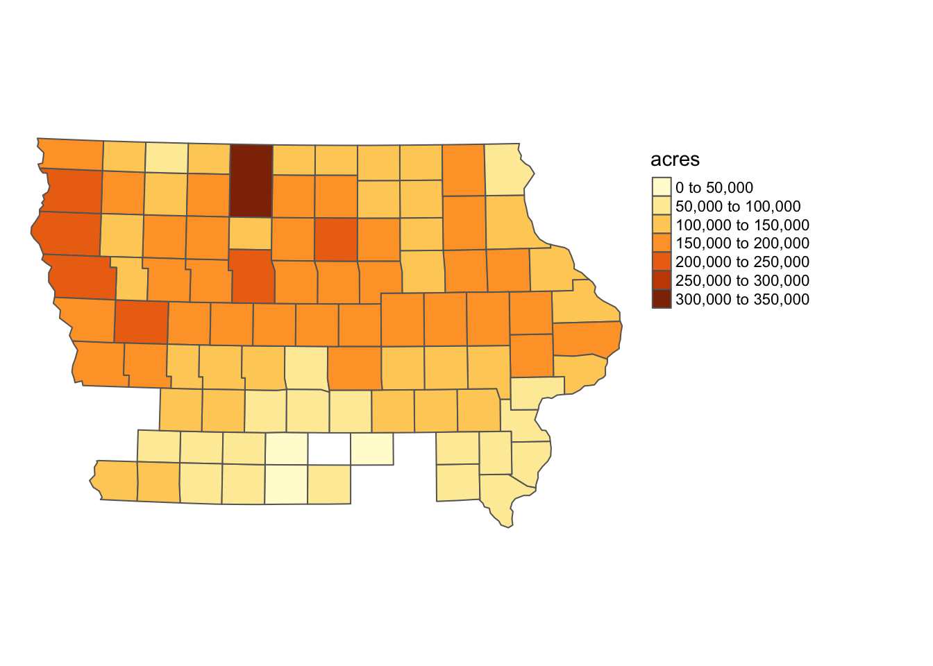
Figure 3.18: Map of Iowa counties color-differentiated by corn planted acreage
Now import the HUC units data:
#--- import HUC units ---#
HUC_IA <- st_read(dsn = "Data", layer = "huc250k") %>%
  dplyr::select(HUC_CODE) %>%
  #--- reproject to the CRS of IA ---#
  st_transform(st_crs(IA_corn)) %>%
  #--- select HUC units that overlaps with IA ---#
  .[IA_corn, ]
Here is the map of HUC units (Figure 3.19):
tm_shape(HUC_IA) +
  tm_polygons() +
  tm_layout(frame = FALSE, legend.outside = TRUE)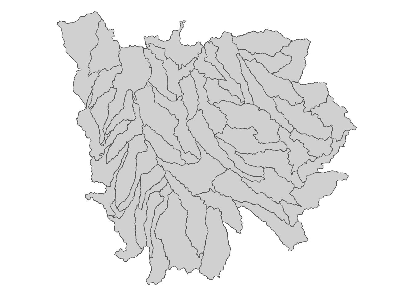
Figure 3.19: Map of HUC units that intersect with Iowa state boundary
Here is a map of Iowa counties with HUC units superimposed on top (Figure 3.20):
tm_shape(IA_corn) +
  tm_polygons(col = "acres") +
tm_shape(HUC_IA) +
  tm_polygons(alpha = 0) +
  tm_layout(frame = FALSE, legend.outside = TRUE)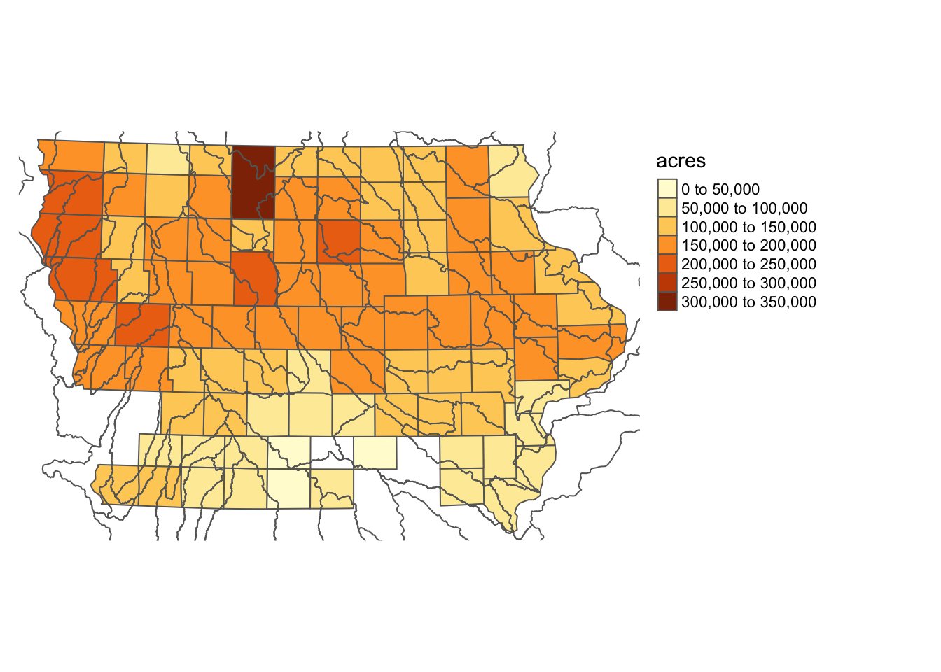
Figure 3.20: Map of HUC units superimposed on the counties in Iowas
Spatial joining will produce the following.
(
HUC_joined <- st_join(HUC_IA, IA_corn)
)
Simple feature collection with 349 features and 4 fields
Geometry type: POLYGON
Dimension: XY
Bounding box: xmin: 154941.7 ymin: 4346327 xmax: 773299.8 ymax: 4907735
Projected CRS: NAD83 / UTM zone 15N
First 10 features:
HUC_CODE county_code year acres geometry
608 10170203 149 2018 226500 POLYGON ((235551.4 4907513,...
608.1 10170203 167 2018 249000 POLYGON ((235551.4 4907513,...
608.2 10170203 193 2018 201000 POLYGON ((235551.4 4907513,...
608.3 10170203 119 2018 184500 POLYGON ((235551.4 4907513,...
621 07020009 063 2018 110500 POLYGON ((408580.7 4880798,...
621.1 07020009 109 2018 304000 POLYGON ((408580.7 4880798,...
621.2 07020009 189 2018 120000 POLYGON ((408580.7 4880798,...
627 10170204 141 2018 167000 POLYGON ((248115.2 4891652,...
627.1 10170204 143 2018 116000 POLYGON ((248115.2 4891652,...
627.2 10170204 167 2018 249000 POLYGON ((248115.2 4891652,...Each of the intersecting HUC-county combinations becomes an observation with its resulting geometry the same as the geometry of the HUC unit. To see this, let’s take a look at one of the HUC units.
The HUC unit with HUC_CODE ==10170203 intersects with four County.
#--- get the HUC unit with `HUC_CODE ==10170203`  ---#
(
temp_HUC_county <- filter(HUC_joined, HUC_CODE == 10170203)
)
Simple feature collection with 4 features and 4 fields
Geometry type: POLYGON
Dimension: XY
Bounding box: xmin: 154941.7 ymin: 4709628 xmax: 248115.2 ymax: 4907735
Projected CRS: NAD83 / UTM zone 15N
HUC_CODE county_code year acres geometry
608 10170203 149 2018 226500 POLYGON ((235551.4 4907513,...
608.1 10170203 167 2018 249000 POLYGON ((235551.4 4907513,...
608.2 10170203 193 2018 201000 POLYGON ((235551.4 4907513,...
608.3 10170203 119 2018 184500 POLYGON ((235551.4 4907513,...Figure 3.21 shows the map of the four observations.
tm_shape(temp_HUC_county) +
  tm_polygons() +
  tm_layout(frame = FALSE)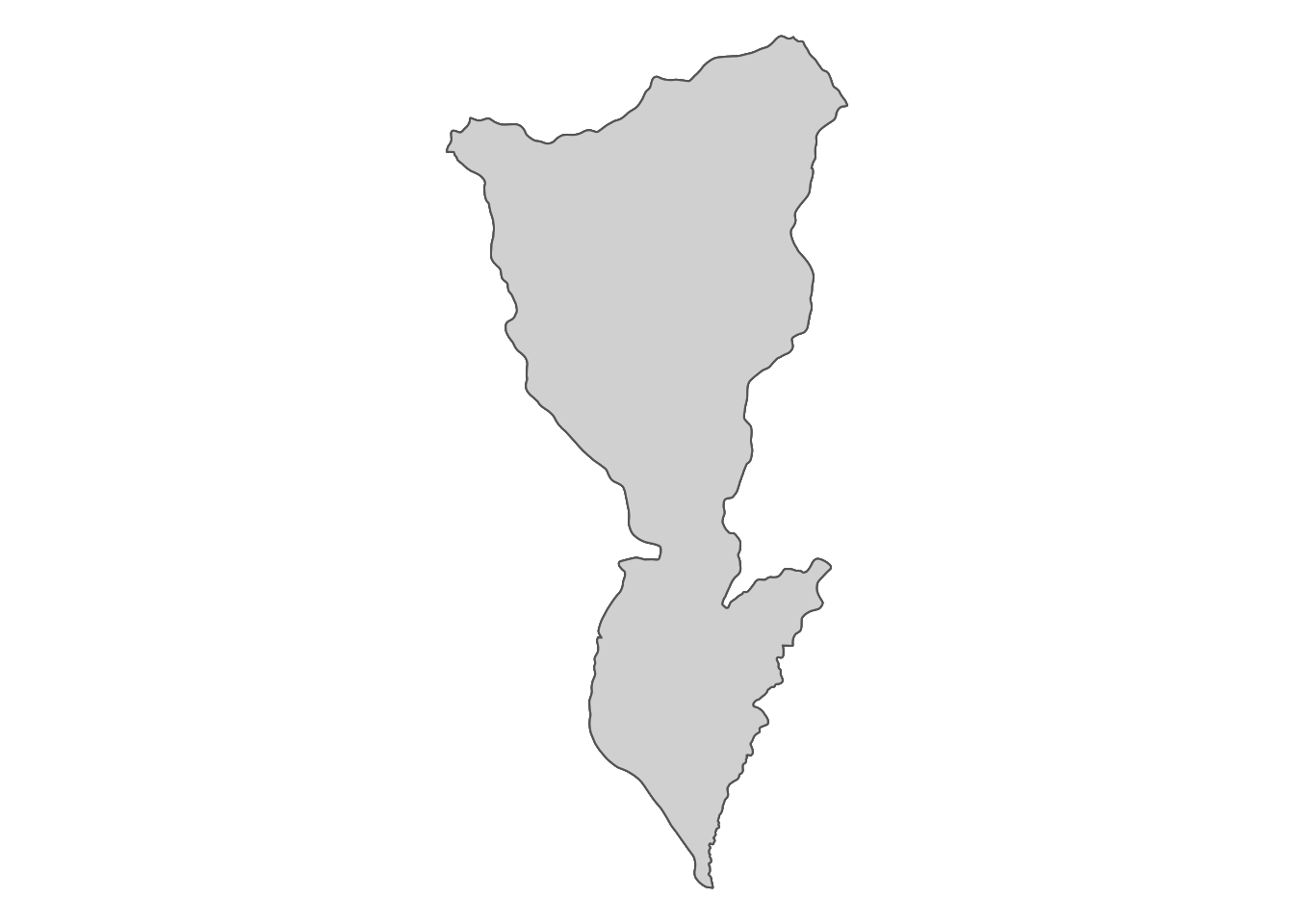
Figure 3.21: Map of the HUC unit
So, all of the four observations have identical geometry, which is the geometry of the HUC unit, meaning that the st_join() did not leave the information about the nature of the intersection of the HUC unit and the four counties. Again, remember that the default option is st_intersects(), which checks whether spatial objects intersect or not, nothing more. If you are just calculating the simple average of corn acres ignoring the degree of spatial overlaps, this is just fine. However, if you would like to calculate area-weighted average, you do not have sufficient information. You will see how to find area-weighted average in the next subsection.
Note that we did not extract any attribute values of the railroads in Chapter 1.4. We just calculated the travel length of the railroads, meaning that the geometry of railroads themselves were of interest instead of values associated with the railroads.↩︎
You can see a practical example of this case in action in Demonstration 1 of Chapter 1.↩︎
While it is unlikely you will face the need to change the topological relation, you could do so using the
joinoption.↩︎You can see a practical example of this case in action in Demonstration 2 of Chapter 1.↩︎
See Chapter 9.1 for how to download Quick Stats data from within R.↩︎
See here for an explanation of what they are. You do not really need to know what HUC units are to understand what’s done in this section.↩︎
Yes, there will be substantial measurement errors as the source polygons (corn acres by county) are large relative to the target polygons (HUC units). But, this serves as a good illustration of a polygon-polygon join.↩︎