2.9 Non-interactive geometrical operations
There are various geometrical operations that are particularly useful for economists. Here, some of the most commonly used geometrical operations are introduced53. You can see the practical use of some of these functions in Chapter 1.4.
2.9.1 st_buffer
st_buffer() creates a buffer around points, lines, or the border of polygons.
Let’s create buffers around points. First, we read well locations data.
#--- read wells location data ---#
urnrd_wells_sf <-
  readRDS("Data/urnrd_wells.rds") %>%
  #--- project to UTM 14N WGS 84 ---#
  st_transform(32614)
Here is the spatial distribution of the wells (Figure 2.4).
tm_shape(urnrd_wells_sf) +
  tm_symbols(col = "red", size = 0.1) +
  tm_layout(frame = FALSE)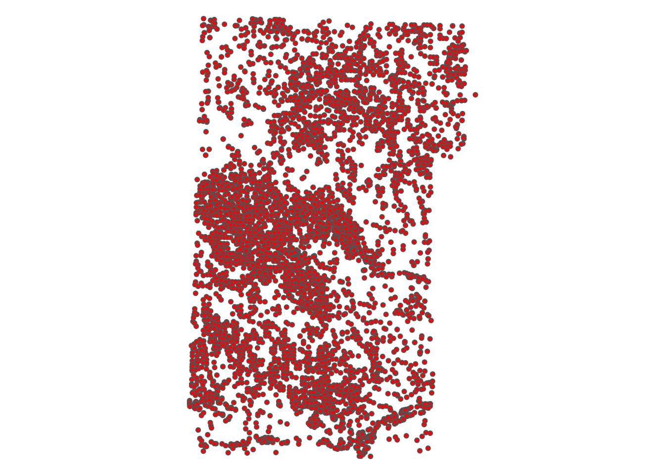
Figure 2.4: Map of the wells
Let’s create buffers around the wells.
#--- create a one-mile buffer around the wells ---#
wells_buffer <- st_buffer(urnrd_wells_sf, dist = 1600)
As you can see, there are many circles around wells with the radius of \(1,600\) meters (Figure 2.5).
tm_shape(wells_buffer) +
  tm_polygons(alpha = 0) +
  tm_shape(urnrd_wells_sf) +
  tm_symbols(col = "red", size = 0.1) +
  tm_layout(frame = NA)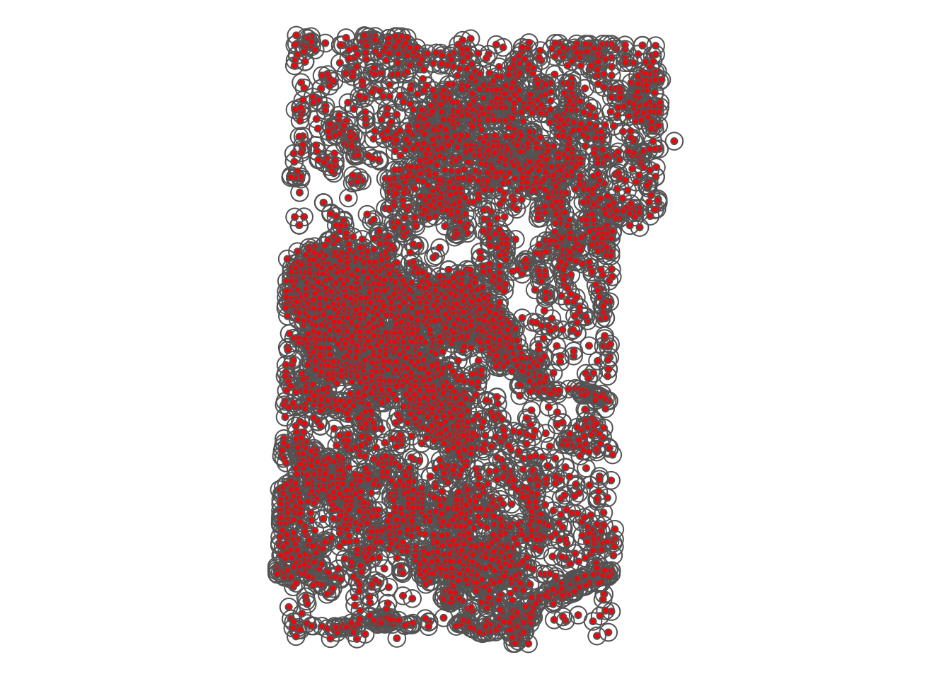
Figure 2.5: Buffers around wells
A practical application of buffer creation can be seen in Chapter 1.1.
We now create buffers around polygons. First, read NE county boundary data and select three counties (Chase, Dundy, and Perkins).
NE_counties <-
  readRDS("Data/NE_county_borders.rds") %>%
  filter(NAME %in% c("Perkins", "Dundy", "Chase")) %>%
  st_transform(32614)
Here is what they look like (Figure 2.6):
tm_shape(NE_counties) +
  tm_polygons("NAME", palette = "RdYlGn", contrast = .3, title = "County") +
  tm_layout(frame = NA)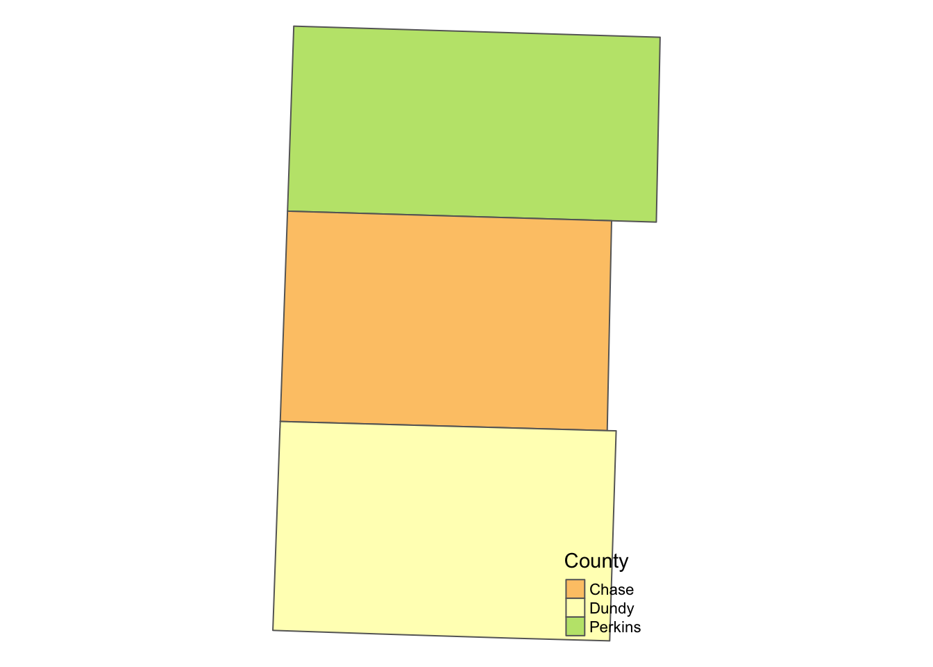
Figure 2.6: Map of the three counties
The following code creates buffers around polygons (see the results in Figure 2.7):
NE_buffer <- st_buffer(NE_counties, dist = 2000)tm_shape(NE_buffer) +
tm_polygons(col = "blue", alpha = 0.2) +
tm_shape(NE_counties) +
tm_polygons("NAME", palette = "RdYlGn", contrast = .3, title = "County") +
tm_layout(
legend.outside = TRUE,
frame = FALSE
)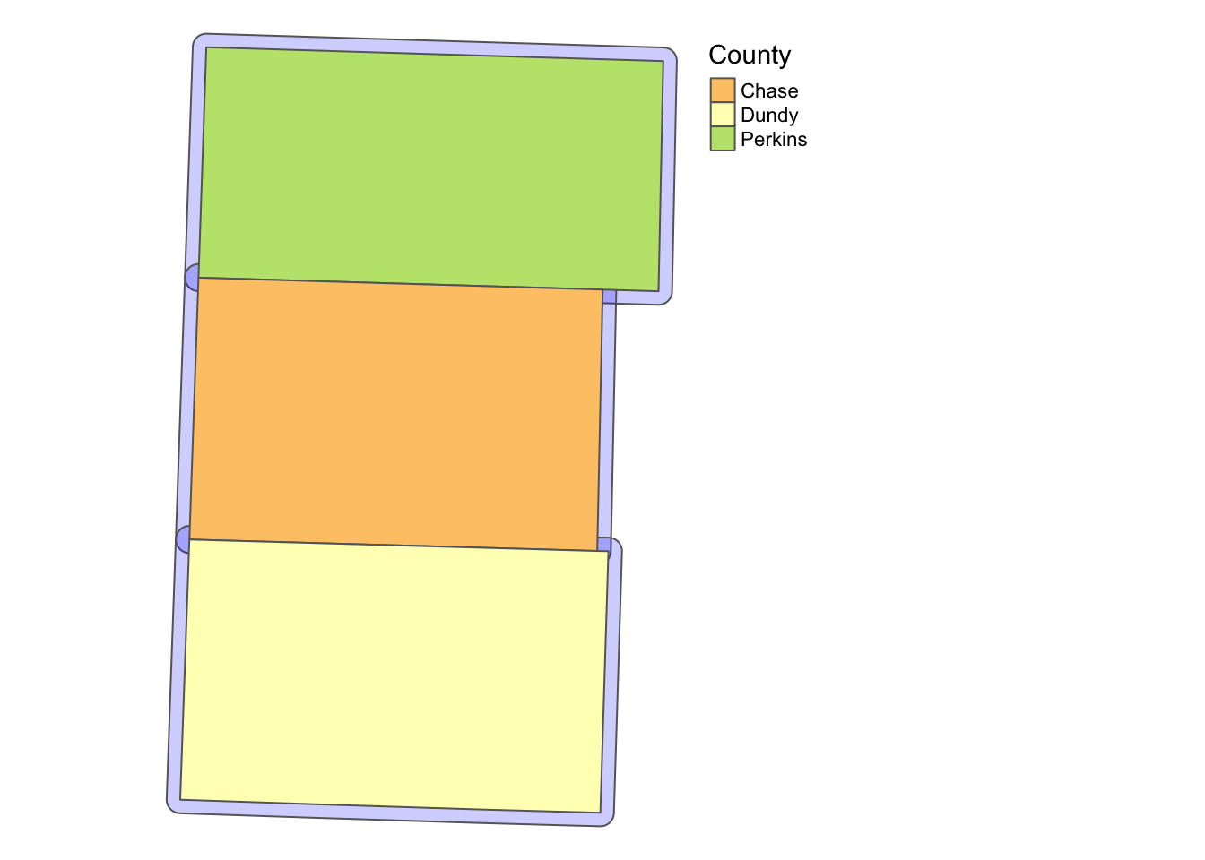
Figure 2.7: Buffers around the three counties
For example, this can be useful to identify observations which are close to the border of political boundaries when you want to take advantage of spatial discontinuity of policies across adjacent political boundaries.
2.9.2 st_area
The st_area() function calculates the area of polygons.
#--- generate area by polygon ---#
(
  NE_counties <- mutate(NE_counties, area = st_area(NE_counties))
)
Simple feature collection with 3 features and 10 fields
Geometry type: MULTIPOLYGON
Dimension: XY
Bounding box: xmin: 239494.1 ymin: 4430632 xmax: 310778.1 ymax: 4543676
Projected CRS: WGS 84 / UTM zone 14N
STATEFP COUNTYFP COUNTYNS AFFGEOID GEOID NAME LSAD ALAND
1 31 135 00835889 0500000US31135 31135 Perkins 06 2287828025
2 31 029 00835836 0500000US31029 31029 Chase 06 2316533447
3 31 057 00835850 0500000US31057 31057 Dundy 06 2381956151
AWATER geometry area
1 2840176 MULTIPOLYGON (((243340.2 45... 2302174854 [m^2]
2 7978172 MULTIPOLYGON (((241201.4 44... 2316908196 [m^2]
3 3046331 MULTIPOLYGON (((240811.3 44... 2389890530 [m^2]Now, as you can see below, the default class of the results of st_area() is units, which does not accept numerical operations.
class(NE_counties$area)[1] "units"So, let’s turn it into double.
(
  NE_counties <- mutate(NE_counties, area = as.numeric(area))
)
Simple feature collection with 3 features and 10 fields
Geometry type: MULTIPOLYGON
Dimension: XY
Bounding box: xmin: 239494.1 ymin: 4430632 xmax: 310778.1 ymax: 4543676
Projected CRS: WGS 84 / UTM zone 14N
STATEFP COUNTYFP COUNTYNS AFFGEOID GEOID NAME LSAD ALAND
1 31 135 00835889 0500000US31135 31135 Perkins 06 2287828025
2 31 029 00835836 0500000US31029 31029 Chase 06 2316533447
3 31 057 00835850 0500000US31057 31057 Dundy 06 2381956151
AWATER geometry area
1 2840176 MULTIPOLYGON (((243340.2 45... 2302174854
2 7978172 MULTIPOLYGON (((241201.4 44... 2316908196
3 3046331 MULTIPOLYGON (((240811.3 44... 2389890530st_area() is useful when you want to find area-weighted average of characteristics after spatially joining two polygon layers using the st_intersection() function (See Chapter 3.3.3).
2.9.3 st_centroid
The st_centroid() function finds the centroid of each polygon.
#--- create centroids ---#
(
  NE_centroids <- st_centroid(NE_counties)
)
Simple feature collection with 3 features and 10 fields
Geometry type: POINT
Dimension: XY
Bounding box: xmin: 271156.7 ymin: 4450826 xmax: 276594.1 ymax: 4525635
Projected CRS: WGS 84 / UTM zone 14N
STATEFP COUNTYFP COUNTYNS AFFGEOID GEOID NAME LSAD ALAND
1 31 135 00835889 0500000US31135 31135 Perkins 06 2287828025
2 31 029 00835836 0500000US31029 31029 Chase 06 2316533447
3 31 057 00835850 0500000US31057 31057 Dundy 06 2381956151
AWATER geometry area
1 2840176 POINT (276594.1 4525635) 2302174854
2 7978172 POINT (271469.9 4489429) 2316908196
3 3046331 POINT (271156.7 4450826) 2389890530Here’s the map of the output (Figure 2.8).
tm_shape(NE_counties) +
  tm_polygons() +
  tm_shape(NE_centroids) +
  tm_symbols(size = 0.5) +
  tm_layout(
    legend.outside = TRUE,
    frame = FALSE
  )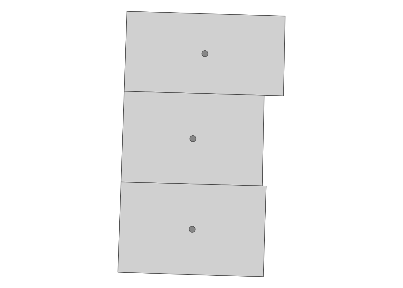
Figure 2.8: The centroids of the polygons
It can be useful when creating a map with labels because the centroid of polygons tend to be a good place to place labels (Figure 2.9).54
tm_shape(NE_counties) +
  tm_polygons() +
  tm_shape(NE_centroids) +
  tm_text("NAME") +
  tm_layout(
    legend.outside = TRUE,
    frame = FALSE
  )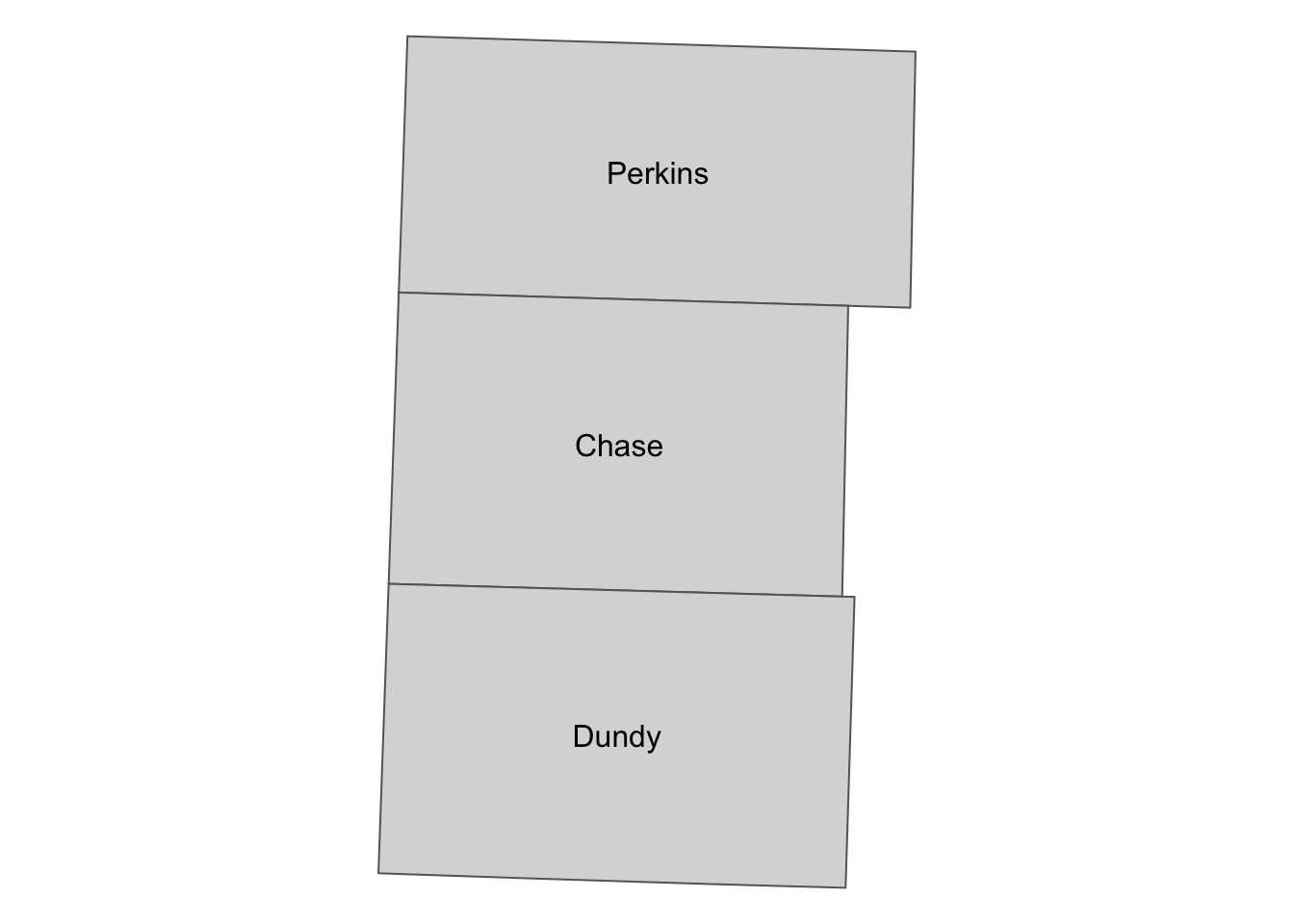
Figure 2.9: County names placed at the centroids of the counties
It may be also useful when you need to calculate the “distance” between polygons.
2.9.4 st_length
We can use st_length() to calculate great circle distances55 of LINESTRING and MULTILINESTRING when they are represented in geodetic coordinates. On the other hand, if they are projected and use a Cartesian coordinate system, it will calculate Euclidean distance. We use U.S. railroad data for a demonstration.
#--- import US railroad data and take only the first 10 of it ---#
(
  a_railroad <- rail_roads <- st_read(dsn = "Data", layer = "tl_2015_us_rails")[1:10, ]
)
Reading layer `tl_2015_us_rails' from data source
`/Users/tmieno2/Dropbox/TeachingUNL/R_as_GIS/Data' using driver `ESRI Shapefile'
Simple feature collection with 180958 features and 3 fields
Geometry type: MULTILINESTRING
Dimension: XY
Bounding box: xmin: -165.4011 ymin: 17.95174 xmax: -65.74931 ymax: 65.00006
Geodetic CRS: NAD83Simple feature collection with 10 features and 3 fields
Geometry type: MULTILINESTRING
Dimension: XY
Bounding box: xmin: -79.74031 ymin: 35.0571 xmax: -79.2377 ymax: 35.51776
Geodetic CRS: NAD83
LINEARID FULLNAME MTFCC geometry
1 11020239500 Norfolk Southern Rlwy R1011 MULTILINESTRING ((-79.47058...
2 11020239501 Norfolk Southern Rlwy R1011 MULTILINESTRING ((-79.46687...
3 11020239502 Norfolk Southern Rlwy R1011 MULTILINESTRING ((-79.66819...
4 11020239503 Norfolk Southern Rlwy R1011 MULTILINESTRING ((-79.46687...
5 11020239504 Norfolk Southern Rlwy R1011 MULTILINESTRING ((-79.74031...
6 11020239575 Seaboard Coast Line RR R1011 MULTILINESTRING ((-79.43695...
7 11020239576 Seaboard Coast Line RR R1011 MULTILINESTRING ((-79.47852...
8 11020239577 Seaboard Coast Line RR R1011 MULTILINESTRING ((-79.43695...
9 11020239589 Aberdeen and Rockfish RR R1011 MULTILINESTRING ((-79.38736...
10 11020239591 Aberdeen and Briar Patch RR R1011 MULTILINESTRING ((-79.53848...#--- check CRS ---#
st_crs(a_railroad)Coordinate Reference System:
User input: NAD83
wkt:
GEOGCRS["NAD83",
DATUM["North American Datum 1983",
ELLIPSOID["GRS 1980",6378137,298.257222101,
LENGTHUNIT["metre",1]]],
PRIMEM["Greenwich",0,
ANGLEUNIT["degree",0.0174532925199433]],
CS[ellipsoidal,2],
AXIS["latitude",north,
ORDER[1],
ANGLEUNIT["degree",0.0174532925199433]],
AXIS["longitude",east,
ORDER[2],
ANGLEUNIT["degree",0.0174532925199433]],
ID["EPSG",4269]]It uses geodetic coordinate system. Let’s calculate the great circle distance of the lines (Chapter 1.4 for a practical use case of this function).
(
  a_railroad <- mutate(a_railroad, length = st_length(a_railroad))
)
Simple feature collection with 10 features and 4 fields
Geometry type: MULTILINESTRING
Dimension: XY
Bounding box: xmin: -79.74031 ymin: 35.0571 xmax: -79.2377 ymax: 35.51776
Geodetic CRS: NAD83
LINEARID FULLNAME MTFCC geometry
1 11020239500 Norfolk Southern Rlwy R1011 MULTILINESTRING ((-79.47058...
2 11020239501 Norfolk Southern Rlwy R1011 MULTILINESTRING ((-79.46687...
3 11020239502 Norfolk Southern Rlwy R1011 MULTILINESTRING ((-79.66819...
4 11020239503 Norfolk Southern Rlwy R1011 MULTILINESTRING ((-79.46687...
5 11020239504 Norfolk Southern Rlwy R1011 MULTILINESTRING ((-79.74031...
6 11020239575 Seaboard Coast Line RR R1011 MULTILINESTRING ((-79.43695...
7 11020239576 Seaboard Coast Line RR R1011 MULTILINESTRING ((-79.47852...
8 11020239577 Seaboard Coast Line RR R1011 MULTILINESTRING ((-79.43695...
9 11020239589 Aberdeen and Rockfish RR R1011 MULTILINESTRING ((-79.38736...
10 11020239591 Aberdeen and Briar Patch RR R1011 MULTILINESTRING ((-79.53848...
length
1 662.0043 [m]
2 658.1026 [m]
3 19953.8571 [m]
4 13880.5060 [m]
5 7183.7286 [m]
6 1062.4649 [m]
7 7832.3375 [m]
8 31773.7700 [m]
9 4544.6795 [m]
10 17101.8581 [m]For the complete list of available geometrical operations under the
sfpackage, see here.↩︎When creating maps with the ggplot2 package, you can use
geom_sf_text()orgeom_sf_label(), which automatically finds where to put texts. See some examples here.↩︎Great circle distance is the shortest distance between two points on the surface of a sphere (earth)↩︎