8.2 Raster data visualization: geom_raster() and geom_stars()

8.2 Raster data visualization: `geom_raster()` and `geom_stars()`

This section shows how to use geom_raster() and geom_stars() to create maps from raster datasets of two object classes: Raster\(^*\) objects from the raster package and stars objects from the stars package. geom_raster does not accept either Raster\(^*\) or stars as the input. Instead, geom_raster() accepts a data.frame with coordinates to create maps. So, it is a two-step procedure

convert raster dataset into a data.frame with coordinates
use geom_raster() to make a map

geom_stars() from the stars package accepts a stars object, and no data transformation is necessary.

We use the following objects that have the same information but come in different object classes for illustration in this section.

Raster as stars

tmax_Jan_09 <- readRDS("Data/tmax_Jan_09_stars.rds")

Raster as RasterStack

tmax_Jan_09_rs <- stack("Data/tmax_Jan_09.tif")

8.2.1 Visualize `Raster`\(^*\) with `geom_raster()`

In order to create maps from the information stored in Raster\(^*\) objects, you first convert them to a regular data.frame using as.data.frame() as follows:

#--- convert to data.frame ---#
tmax_Jan_09_df <-
  as.data.frame(tmax_Jan_09_rs, xy = TRUE) %>%
  #--- remove cells with NA for any of the layers ---#
  na.omit() %>%
  #--- change the variable names ---#
  setnames(
    paste0("tmax_Jan_09.", 1:5),
    seq(ymd("2009-01-01"), ymd("2009-01-05"), by = "days") %>%
      as.character()
  )

#--- take a look ---#
head(tmax_Jan_09_df)

              x        y 2009-01-01 2009-01-02 2009-01-03 2009-01-04 2009-01-05
17578 -95.12500 49.41667    -12.863    -11.455    -17.516    -12.755    -26.446
18982 -95.16667 49.37500    -12.698    -11.441    -17.436    -12.672    -25.889
18983 -95.12500 49.37500    -12.921    -11.611    -17.589    -12.830    -26.544
18984 -95.08333 49.37500    -13.074    -11.827    -17.684    -12.913    -26.535
18985 -95.04167 49.37500    -13.591    -12.220    -17.920    -12.684    -25.780
18986 -95.00000 49.37500    -13.688    -12.177    -17.911    -12.548    -25.424

The xy = TRUE option adds the coordinates of the centroid of the raster cells, and na.omit() removes cells that are outside of the Kansas border and have NA values. Notice that each band comprises a column in the data.frame.

Once the conversion is done, you can use geom_raster() to create a map. Unlike geom_sf(), you need to supply the variables names for the geographical coordinates (here x for longitude and y for latitude). Further, you also need to specify which variable to use for fill color differentiation.

(
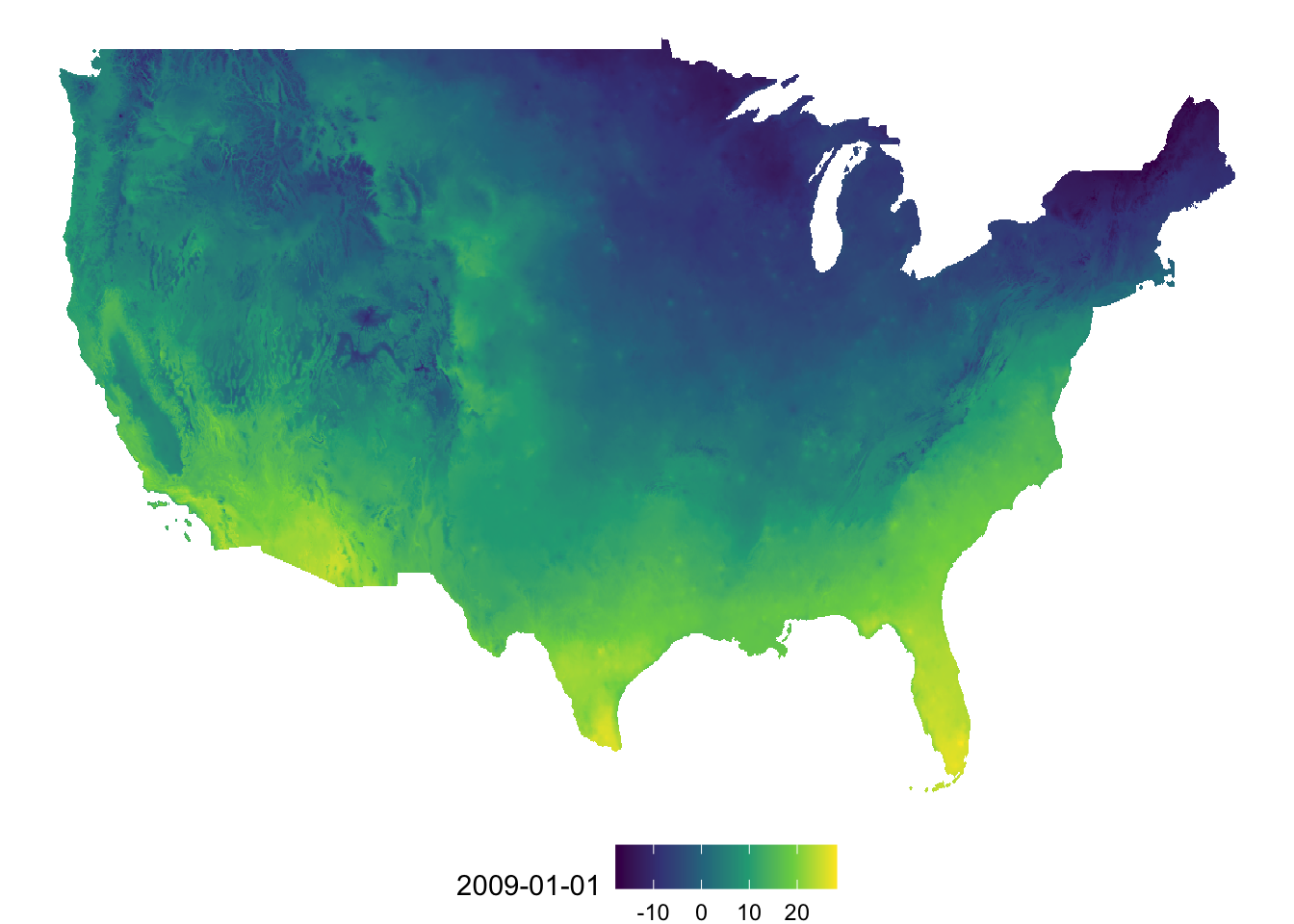
  g_tmax_map <- ggplot(data = tmax_Jan_09_df) +
    geom_raster(aes(x = x, y = y, fill = `2009-01-01`)) +
    scale_fill_viridis_c() +
    theme_void() +
    theme(
      legend.position = "bottom"
    )
)

You can add coord_equal() so that one degree in latitude and longitude are the same length on the map. Of course, one degree in longitude and one degree in latitude are not the same length for US. However, distortion is smaller compared to the default at least.

g_tmax_map + coord_equal()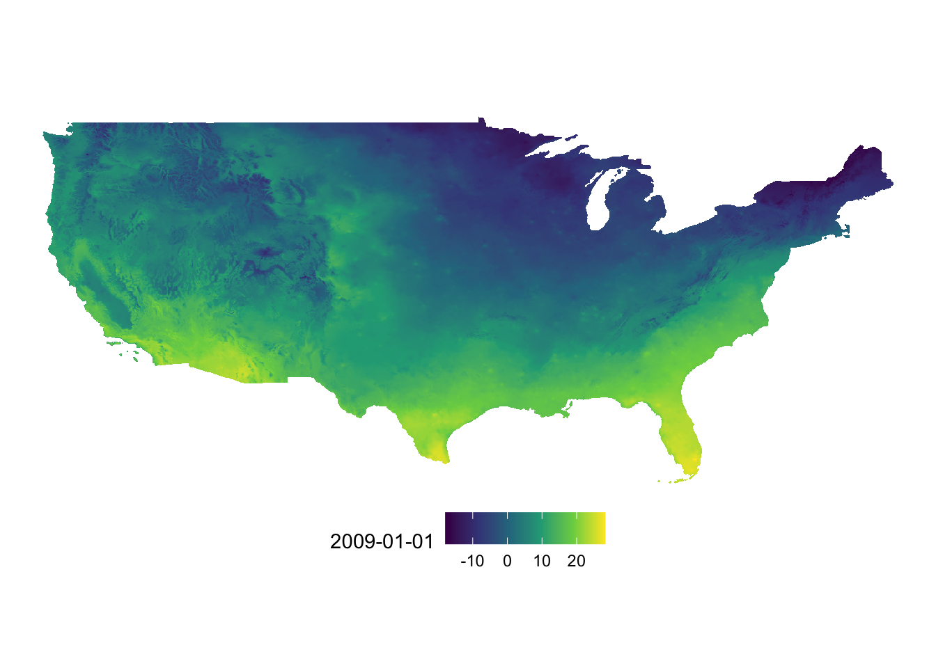

We only visualized tmax data for one day (layer.1) out of five days of tmax records. To present all of them at the same time we can facet using facet_wrap(). However, before we do that we need to have the data in a long format like this:

tmax_long_df <- 
  tmax_Jan_09_df %>%
  pivot_longer(
    c(-x, -y),
    names_to = "date",
    values_to = "tmax"
  )

#--- take a look ---#
head(tmax_long_df)

# A tibble: 6 × 4
      x     y date        tmax
  <dbl> <dbl> <chr>      <dbl>
1 -95.1  49.4 2009-01-01 -12.9
2 -95.1  49.4 2009-01-02 -11.5
3 -95.1  49.4 2009-01-03 -17.5
4 -95.1  49.4 2009-01-04 -12.8
5 -95.1  49.4 2009-01-05 -26.4
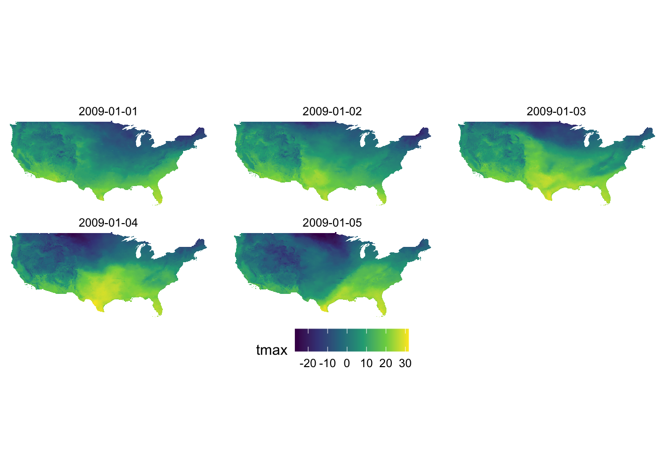
6 -95.2  49.4 2009-01-01 -12.7

Let’s now use facet_wrap() to create a series of tmax maps.

ggplot() +
  geom_raster(data = tmax_long_df, aes(x = x, y = y, fill = tmax)) +
  facet_wrap(date ~ .) +
  coord_equal() +
  scale_fill_viridis_c() +
  theme_void() +
  theme(
    legend.position = "bottom"
  )

8.2.2 Visualize `stars` with `geom_raster()`

Similarly with Raster\(^*\) objects, we first need to convert a stars to a regular data.frame using as.data.frame() as follows:

#--- converting to a data.frame ---#
tmax_long_df <- as.data.frame(tmax_Jan_09, xy = TRUE) %>%
  na.omit()

#--- take a look ---#
head(tmax_Jan_09_df)

              x        y 2009-01-01 2009-01-02 2009-01-03 2009-01-04 2009-01-05
17578 -95.12500 49.41667    -12.863    -11.455    -17.516    -12.755    -26.446
18982 -95.16667 49.37500    -12.698    -11.441    -17.436    -12.672    -25.889
18983 -95.12500 49.37500    -12.921    -11.611    -17.589    -12.830    -26.544
18984 -95.08333 49.37500    -13.074    -11.827    -17.684    -12.913    -26.535
18985 -95.04167 49.37500    -13.591    -12.220    -17.920    -12.684    -25.780
18986 -95.00000 49.37500    -13.688    -12.177    -17.911    -12.548    -25.424

One key difference from the conversion of Raster\(^*\) objects is that the data.frame is already in the long format, which means that you can immediately make faceted figures like this:

ggplot() +
  geom_raster(data = tmax_long_df, aes(x = x, y = y, fill = tmax)) +
  facet_wrap(date ~ .) +
  coord_equal() +
  scale_fill_viridis_c() +
  theme_void() +
  theme(
    legend.position = "bottom"
  )

8.2.3 Visualize `stars` with `geom_stars()`

We saw above that geom_raster() requires converting a stars object to a data.frame first before creating a map. geom_stars() from the stars package lets you use a stars object directly to easily create a map under the ggplot2 framework. geom_stars() works just like geom_sf(). All you need to do is supply a stars object to geom_stars() as data.

ggplot() +
  geom_stars(data = tmax_Jan_09) +
  theme_void()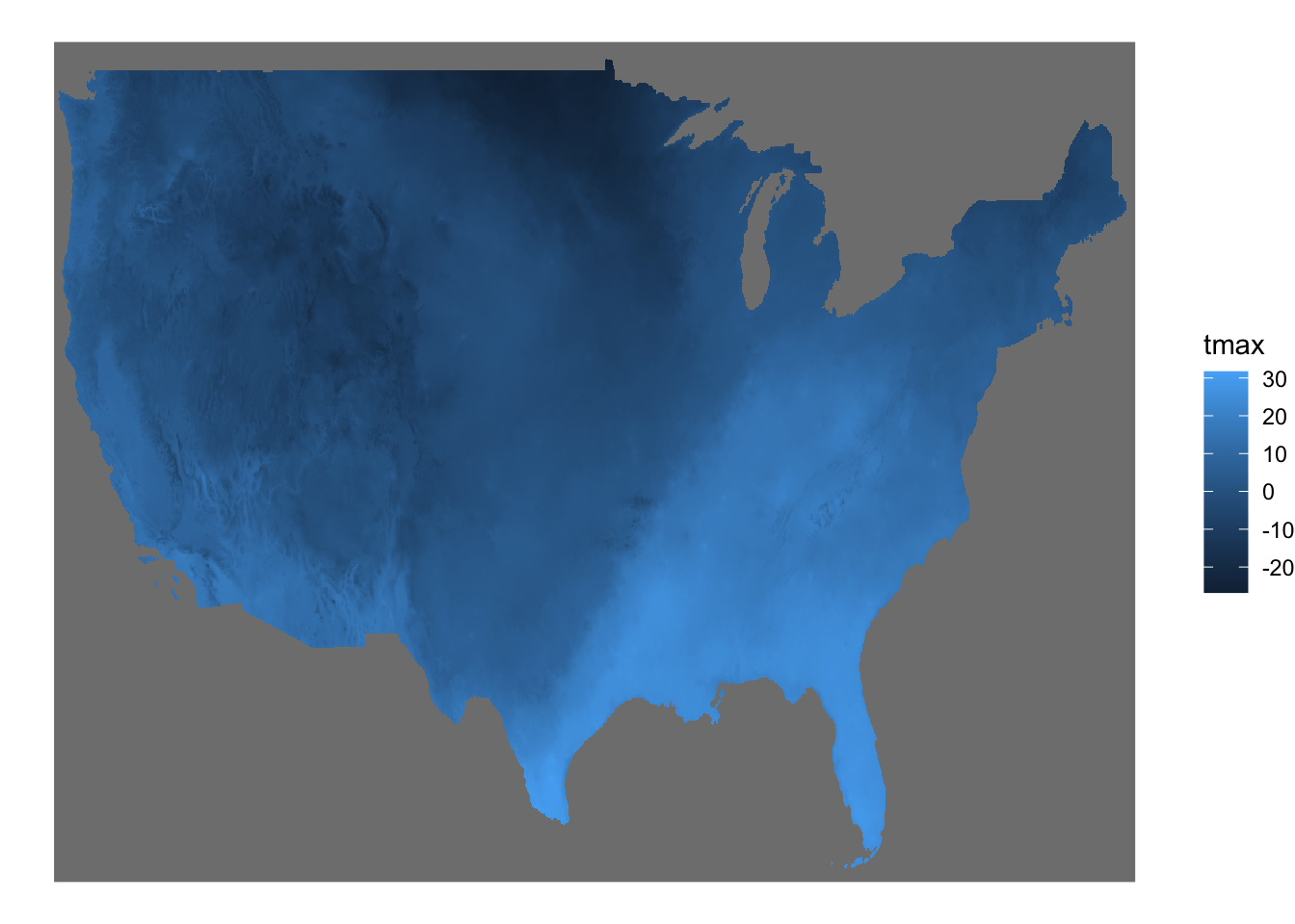

The fill color of the raster cells are automatically set to the attribute (here tmax) as if aes(fill = tmax). It is a good idea to add coord_equal() because of the same issue we saw with geom_raster().

ggplot() +
  geom_stars(data = tmax_Jan_09) +
  theme_void() +
  coord_equal()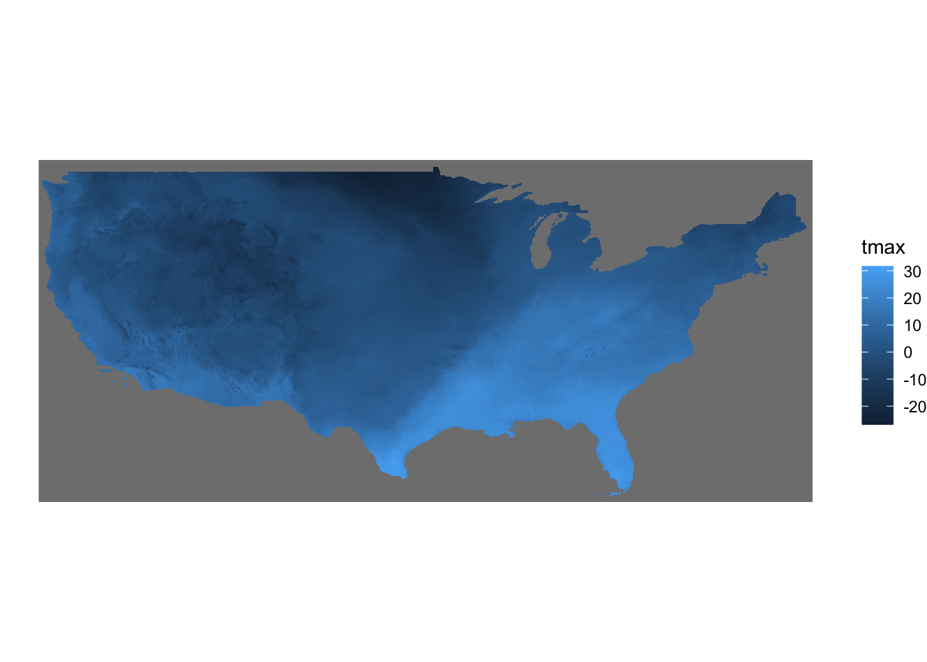

By default, geom_stars() plots only the first band. In order to present all the layers at the same time, you can add facet_wrap( ~ x) where x is the name of the third dimension of the stars object (date here).

ggplot() +
  geom_stars(data = tmax_Jan_09) +
  facet_wrap(~date) +
  coord_equal() +
  theme_void()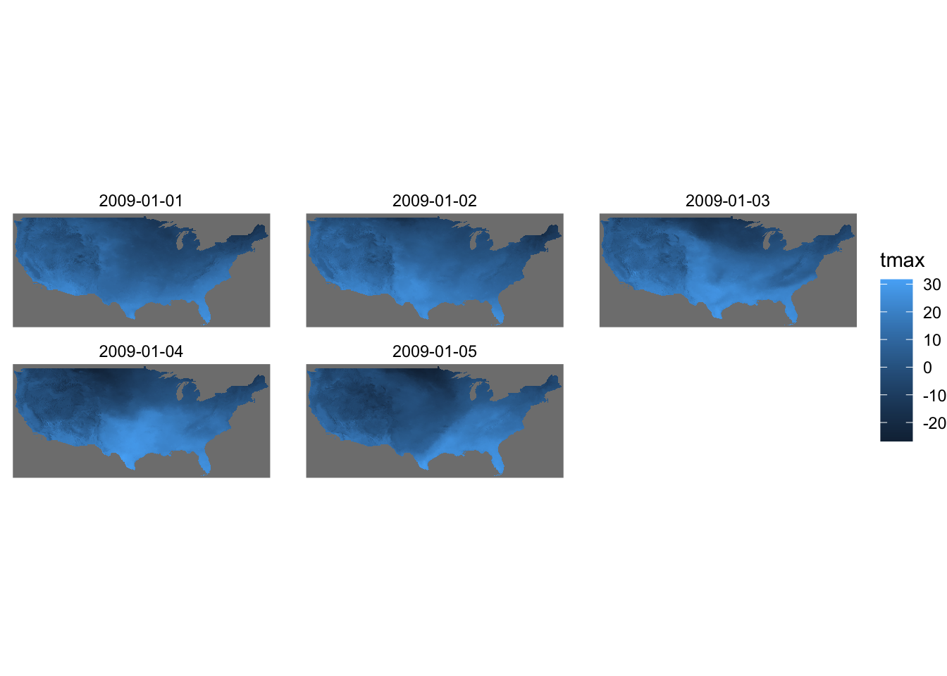

8.2.4 adding `geom_sf()` layers

You can easily add geom_sf() layers to a map created with geom_raster() or geom_stars(). Let’s crop the tmax data to Kansas and create a map of tmax values displayed on top of the Kansas county borders.

#--- crop to KS ---#
KS_tmax_Jan_09_stars <- tmax_Jan_09 %>%
  st_crop(., KS_county)

#--- convert to a df ---#
KS_tmax_Jan_09_df <- as.data.frame(KS_tmax_Jan_09_stars, xy = TRUE) %>%
  na.omit()

8.2.4.1 adding `geom_sf()` to a map with `geom_raster()`

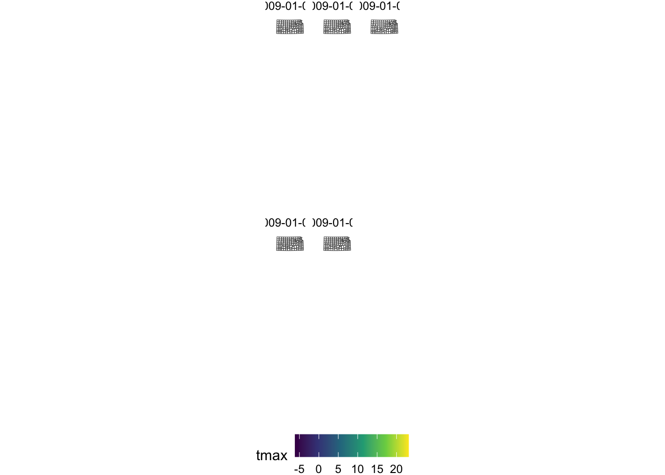
ggplot() +
  geom_raster(data = KS_tmax_Jan_09_df, aes(x = x, y = y, fill = tmax)) +
  geom_sf(data = KS_county, fill = NA) +
  facet_wrap(date ~ .) +
  scale_fill_viridis_c() +
  theme_void() +
  theme(
    legend.position = "bottom"
  )

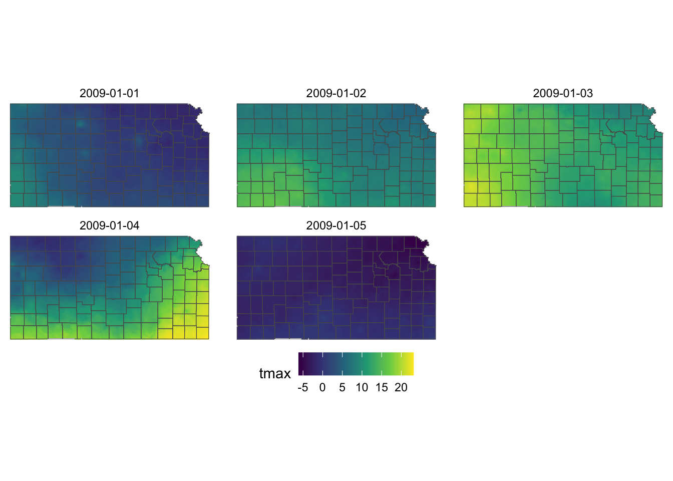
Notice that coord_equal() is not necessary in the above code. Indeed, if you try to add coord_equal(), you will have an error.

ggplot() +
  geom_raster(data = KS_tmax_Jan_09_df, aes(x = x, y = y, fill = tmax)) +
  geom_sf(data = KS_county, fill = NA) +
  facet_wrap(date ~ .) +
  coord_equal() +
  scale_fill_viridis_c() +
  theme_void() +
  theme(
    legend.position = "bottom"
  )

Error in `f()`:
! geom_sf() must be used with coord_sf()

Further, the original stars or Raster\(^*\) must have the same CRS as the sf objects. The following code transforms the CRS of KS_county to 32614 and try to plot them together.

ggplot() +
  geom_raster(data = KS_tmax_Jan_09_df, aes(x = x, y = y, fill = tmax)) +
  geom_sf(data = st_transform(KS_county, 32614), fill = NA) +
  facet_wrap(date ~ .) +
  scale_fill_viridis_c() +
  theme_void() +
  theme(
    legend.position = "bottom"
  )

When plotting multiple sf objects, the CRS for the map was set to the CRS of the sf objects used for the first geom_sf() layer, and the rest of the sf objects followed suit. That is not the case here.

8.2.4.2 adding `geom_sf()` to a map with `geom_stars()`

This is basically the same as the case with geom_stars()

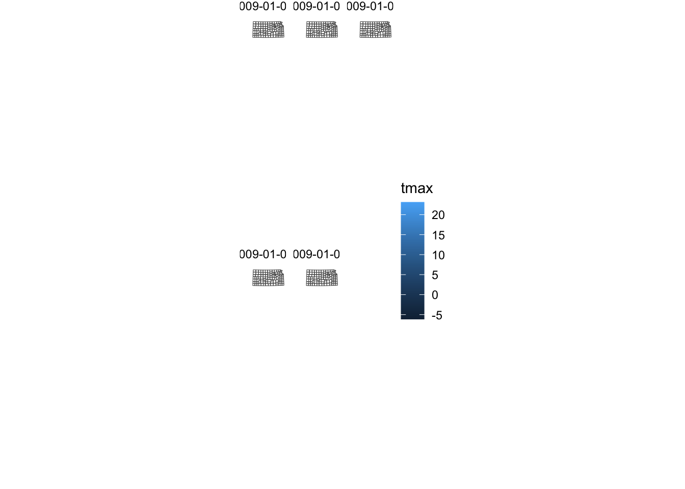
ggplot() +
  geom_stars(data = KS_tmax_Jan_09_stars) +
  geom_sf(data = KS_county, fill = NA) +
  facet_wrap(~date) +
  theme_void()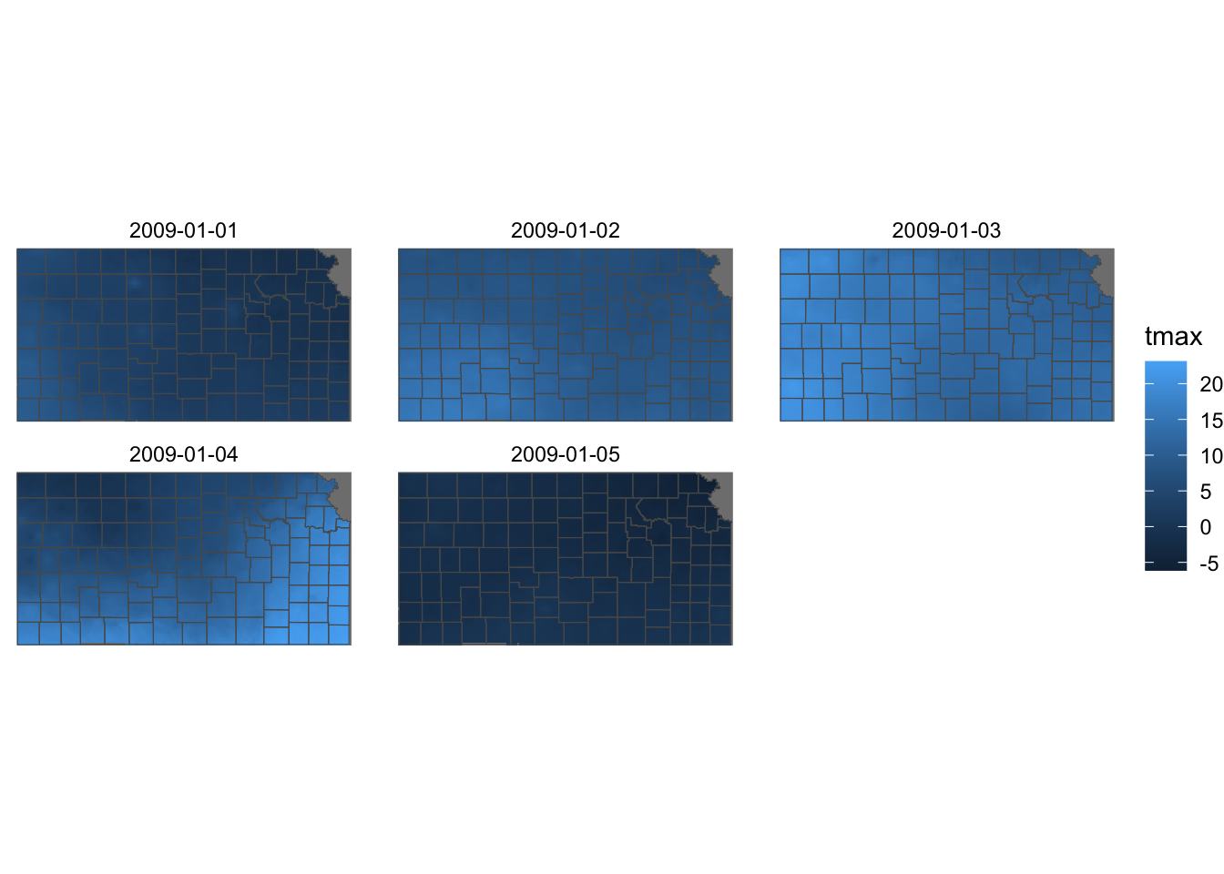

Just like the case with geom_raster(), coord_equal() is not necessary and the stars and sf objects must have the same CRS.

ggplot() +
  geom_stars(data = KS_tmax_Jan_09_stars) +
  geom_sf(data = st_transform(KS_county, 32614), fill = NA) +
  facet_wrap(~date) +
  theme_void()