7.6 dplyr-like operations

7.6 `dplyr`-like operations

You can use the dplyr language to do basic data operations on stars objects.

7.6.1 `filter()`

The filter() function allows you to subset data by dimension values: x, y, and band (here date).

spatial filtering

library(tidyverse)

#--- longitude greater than -100 ---#
filter(ppt_m1_y09_stars, x > -100) %>% plot()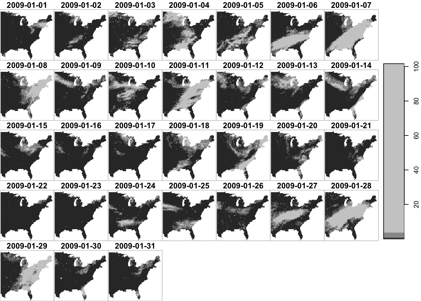

#--- latitude less than 40 ---#
filter(ppt_m1_y09_stars, y < 40) %>% plot()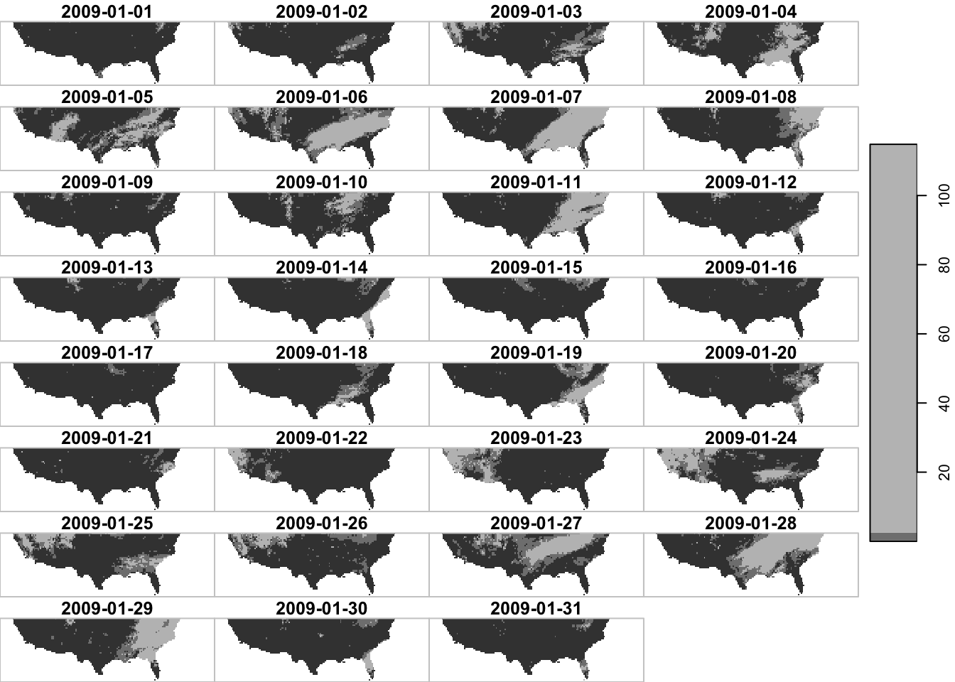

temporal filtering

Finally, since the date dimension is in Date, you can use Date math to filter the data.⁸⁵

#--- dates after 2009-01-15  ---#
filter(ppt_m1_y09_stars, date > ymd("2009-01-21")) %>% plot()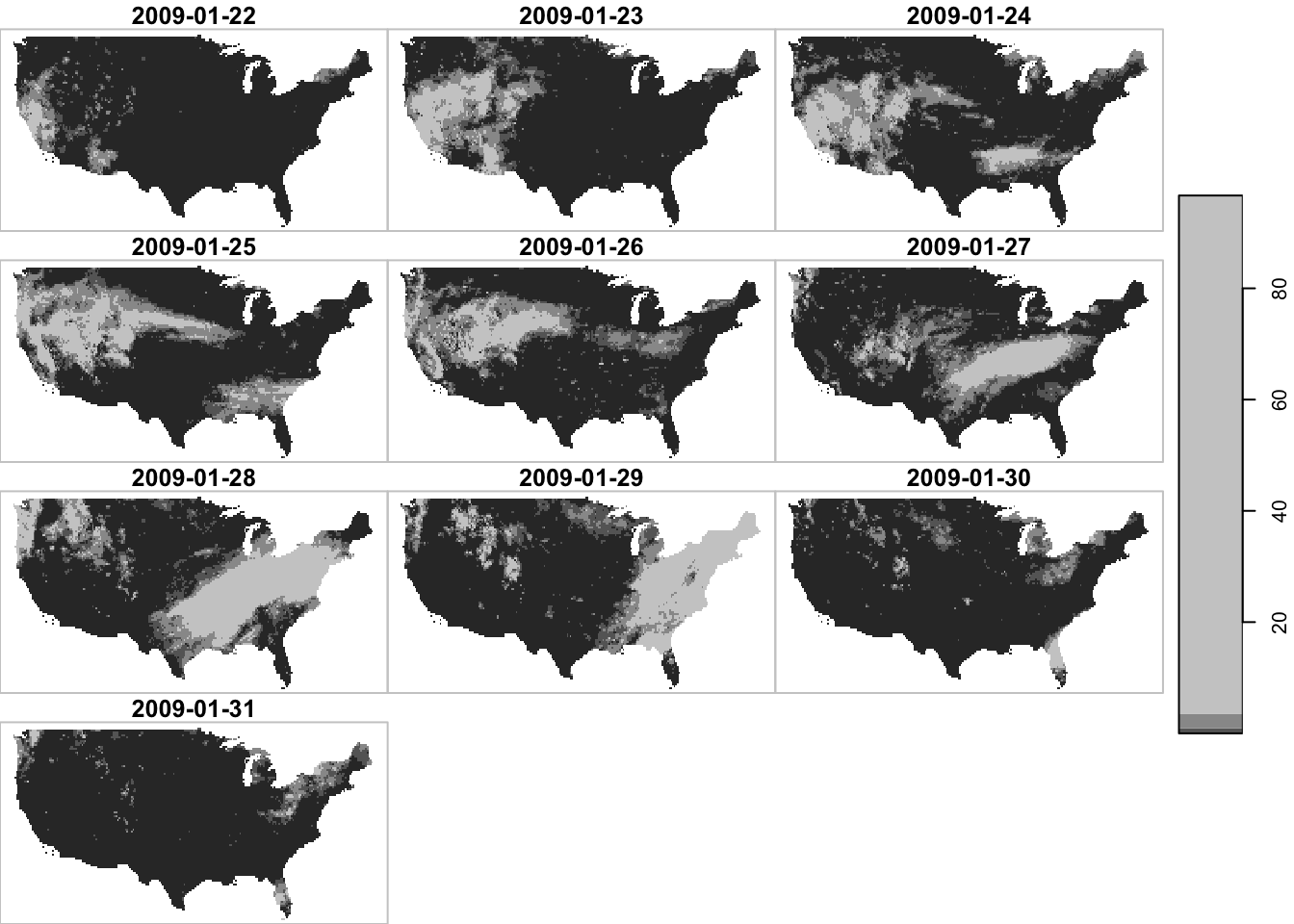

filter by attribute?

Just in case you are wondering. You cannot filter by attribute.

filter(ppt_m1_y09_stars, ppt > 20)

Error in `glubort()`:
! ``~``, `ppt > 20` must refer to exactly one dimension, not ``

7.6.2 `select()`

The select() function lets you pick certain attributes.

select(prcp_tmax_PRISM_m8_y09, ppt)

stars object with 3 dimensions and 1 attribute
attribute(s):
     Min. 1st Qu. Median     Mean 3rd Qu.   Max.
ppt     0       0      0 1.292334   0.011 30.851
dimension(s):
     from to     offset      delta refsys point values x/y
x       1 20   -121.729  0.0416667  NAD83 FALSE   NULL [x]
y       1 20    46.6458 -0.0416667  NAD83 FALSE   NULL [y]
date    1 10 2009-08-11     1 days   Date    NA   NULL

7.6.3 `mutate()`

You can mutate attributes using the mutate() function. For example, this can be useful to calculate NDVI in a stars object that has Red and NIR (spectral reflectance measurements in the red and near-infrared regions) as attributes. Here, we just simply convert the unit of precipitation from mm to inches.

#--- mm to inches ---#
mutate(prcp_tmax_PRISM_m8_y09, ppt = ppt * 0.0393701)

stars object with 3 dimensions and 2 attributes
attribute(s):
       Min.  1st Qu. Median       Mean      3rd Qu.      Max.
ppt   0.000  0.00000  0.000  0.0508793 4.330711e-04  1.214607
tmax  1.833 17.55575 21.483 22.0354348 2.654275e+01 39.707001
dimension(s):
     from to     offset      delta refsys point values x/y
x       1 20   -121.729  0.0416667  NAD83 FALSE   NULL [x]
y       1 20    46.6458 -0.0416667  NAD83 FALSE   NULL [y]
date    1 10 2009-08-11     1 days   Date    NA   NULL

7.6.4 `pull()`

You can extract attribute values using pull().

#--- tmax values of the 1st date layer ---#
pull(prcp_tmax_PRISM_m8_y09["tmax",,,1], "tmax")

, , 1

        [,1]   [,2]   [,3]   [,4]   [,5]   [,6]   [,7]   [,8]   [,9]  [,10]
 [1,] 25.495 27.150 22.281 19.553 21.502 19.616 21.664 24.458 21.712 19.326
 [2,] 27.261 27.042 21.876 19.558 19.141 19.992 18.694 24.310 21.094 20.032
 [3,] 27.568 21.452 23.220 19.428 18.974 19.366 20.293 24.418 20.190 21.127
 [4,] 23.310 20.357 20.111 21.380 19.824 19.638 22.135 20.885 20.121 18.396
 [5,] 19.571 20.025 18.407 19.142 19.314 22.759 22.652 19.566 18.817 16.065
 [6,] 17.963 16.581 17.121 16.716 19.680 20.521 17.991 18.007 17.430 14.586
 [7,] 20.911 19.202 16.309 14.496 17.429 19.083 18.509 18.723 17.645 16.415
 [8,] 17.665 16.730 17.691 14.370 16.849 18.413 17.787 20.000 19.319 18.401
 [9,] 16.795 18.091 20.460 16.405 18.331 19.005 19.142 21.226 21.184 19.520
[10,] 19.208 19.624 17.210 19.499 18.492 20.854 18.684 19.811 22.058 19.923
[11,] 23.148 18.339 19.676 20.674 18.545 21.126 19.013 19.722 21.843 21.271
[12,] 23.254 21.279 21.921 19.894 19.445 21.499 19.765 20.742 21.560 22.989
[13,] 23.450 21.956 19.813 18.970 20.173 20.567 21.152 20.932 19.836 20.347
[14,] 24.075 21.120 20.166 19.177 20.428 20.908 21.060 19.832 19.764 19.981
[15,] 24.318 20.943 20.024 20.022 19.040 19.773 20.452 20.152 20.321 20.304
[16,] 22.538 19.461 20.100 21.149 19.958 20.486 20.535 20.445 21.564 21.493
[17,] 20.827 20.192 21.165 22.369 21.488 22.031 21.552 21.089 21.687 23.375
[18,] 21.089 21.451 22.692 21.793 22.160 23.049 22.562 22.738 23.634 24.697
[19,] 22.285 22.992 23.738 23.497 24.255 25.177 25.411 24.324 24.588 26.032
[20,] 23.478 23.584 24.589 24.719 26.114 26.777 27.310 26.643 26.516 26.615
       [,11]  [,12]  [,13]  [,14]  [,15]  [,16]  [,17]  [,18]  [,19]  [,20]
 [1,] 24.845 23.211 21.621 23.180 21.618 21.322 22.956 23.749 23.162 25.746
 [2,] 24.212 21.820 21.305 22.960 22.806 22.235 23.604 23.689 25.597 25.933
 [3,] 20.879 20.951 22.280 23.536 23.455 22.537 24.760 23.587 26.170 24.764
 [4,] 17.435 18.681 22.224 24.122 25.828 25.604 25.298 22.817 24.438 24.835
 [5,] 14.186 17.789 20.624 23.416 26.059 27.571 25.158 24.201 26.001 26.235
 [6,] 10.188 15.632 19.907 22.660 25.268 27.469 27.376 27.488 27.278 27.558
 [7,] 14.797 15.933 19.204 21.641 23.107 25.626 26.990 25.838 26.906 27.247
 [8,] 17.325 18.299 19.691 21.553 21.840 23.754 26.099 25.270 26.282 26.981
 [9,] 19.322 19.855 20.489 22.597 23.614 25.873 26.906 26.368 26.332 25.844
[10,] 20.241 21.800 22.111 24.128 25.765 27.105 27.200 25.491 26.306 25.663
[11,] 23.398 24.090 24.884 25.596 26.545 27.014 26.464 25.708 25.742 25.336
[12,] 22.576 21.996 23.874 26.447 26.955 26.871 25.533 25.576 25.610 25.902
[13,] 22.023 22.358 24.996 26.185 27.249 25.617 25.623 25.600 25.433 26.681
[14,] 20.974 23.533 25.388 25.975 27.316 26.199 26.090 25.920 25.767 27.956
[15,] 20.982 23.632 24.703 25.539 26.515 27.133 27.407 27.518 27.149 28.506
[16,] 22.500 24.012 25.282 25.751 25.212 25.290 26.058 28.258 28.290 29.842
[17,] 23.024 24.381 25.157 25.259 24.829 24.183 25.632 26.947 28.601 29.589
[18,] 24.016 24.425 24.965 24.930 24.482 23.274 25.412 26.733 28.494 29.656
[19,] 24.065 24.105 24.145 24.318 23.912 22.782 25.039 26.554 28.184 29.012
[20,] 23.979 24.321 23.477 22.135 22.395 22.189 24.944 26.542 27.923 28.849

Of course, this is possible only because we have assigned date values to the band dimension above.↩︎

7.6.1 filter()

7.6.2 select()

7.6.3 mutate()

7.6.4 pull()