1.1 Demonstration 1: The impact of groundwater pumping on depth to water table

1.1.1 Project Overview

---

Objective:

• Understand the impact of groundwater pumping on groundwater level.

---

Datasets

• Groundwater pumping by irrigation wells in Chase, Dundy, and Perkins Counties in the southwest corner of Nebraska
• Groundwater levels observed at USGS monitoring wells located in the three counties and retrieved from the National Water Information System (NWIS) maintained by USGS using the dataRetrieval package.

---

Econometric Model

In order to achieve the project objective, we will estimate the following model:

\[ y_{i,t} - y_{i,t-1} = \alpha + \beta gw_{i,t-1} + v \]

where \(y_{i,t}\) is the depth to groundwater table¹⁰ in March¹¹ in year \(t\) at USGS monitoring well \(i\), and \(gw_{i,t-1}\) is the total amount of groundwater pumping that happened within the 2-mile radius of the monitoring well \(i\).

---

GIS tasks

• read an ESRI shape file as an sf (spatial) object
  • use sf::st_read()
• download depth to water table data using the dataRetrieval package developed by USGS
  • use dataRetrieval::readNWISdata() and dataRetrieval::readNWISsite()
• create a buffer around USGS monitoring wells
  • use sf::st_buffer()
• convert a regular data.frame (non-spatial) with geographic coordinates into an sf (spatial) objects
  • use sf::st_as_sf() and sf::st_set_crs()
• reproject an sf object to another CRS
  • use sf::st_transform()
• identify irrigation wells located inside the buffers and calculate total pumping
  • use sf::st_join()
• create maps
  • use the tmap package

---

Preparation for replication

Run the following code to install or load (if already installed) the pacman package, and then install or load (if already installed) the listed package inside the pacman::p_load() function.

if (!require("pacman")) install.packages("pacman")
pacman::p_load(
  sf, # vector data operations
  dplyr, # data wrangling
  dataRetrieval, # download USGS NWIS data
  lubridate, # Date object handling
  modelsummary, # regression table generation
  lfe # fast regression with many fixed effects
)

1.1.2 Project Demonstration

The geographic focus of the project is the southwest corner of Nebraska consisting of Chase, Dundy, and Perkins County (see Figure 1.1 for their locations within Nebraska). Let’s read a shape file of the three counties represented as polygons. We will use it later to spatially filter groundwater level data downloaded from NWIS.

three_counties <-
  st_read(dsn = "Data", layer = "urnrd") %>%
  #--- project to WGS84/UTM 14N ---#
  st_transform(32614)

Reading layer `urnrd' from data source 
  `/Users/tmieno2/Dropbox/TeachingUNL/R_as_GIS/Data' using driver `ESRI Shapefile'
Simple feature collection with 3 features and 1 field
Geometry type: POLYGON
Dimension:     XY
Bounding box:  xmin: -102.0518 ymin: 40.00257 xmax: -101.248 ymax: 41.00395
Geodetic CRS:  NAD83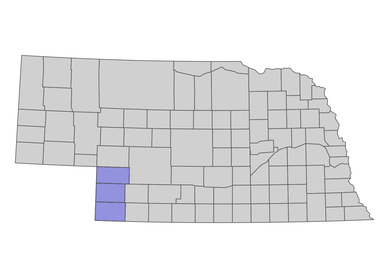

Figure 1.1: The location of Chase, Dundy, and Perkins County in Nebraska

---

We have already collected groundwater pumping data, so let’s import it.

#--- groundwater pumping data ---#
(
  urnrd_gw <- readRDS("Data/urnrd_gw_pumping.rds")
)

       well_id year  vol_af      lon     lat
    1:    1706 2007 182.566 245322.3 4542717
    2:    2116 2007  46.328 245620.9 4541125
    3:    2583 2007  38.380 245660.9 4542523
    4:    2597 2007  70.133 244816.2 4541143
    5:    3143 2007 135.870 243614.0 4541579
   ---                                      
18668:    2006 2012 148.713 284782.5 4432317
18669:    2538 2012 115.567 284462.6 4432331
18670:    2834 2012  15.766 283338.0 4431341
18671:    2834 2012 381.622 283740.4 4431329
18672:    4983 2012      NA 284636.0 4432725

well_id is the unique irrigation well identifier, and vol_af is the amount of groundwater pumped in acre-feet. This dataset is just a regular data.frame with coordinates. We need to convert this dataset into a object of class sf so that we can later identify irrigation wells located within a 2-mile radius of USGS monitoring wells (see Figure 1.2 for the spatial distribution of the irrigation wells).

urnrd_gw_sf <-
  urnrd_gw %>%
  #--- convert to sf ---#
  st_as_sf(coords = c("lon", "lat")) %>%
  #--- set CRS WGS UTM 14 (you need to know the CRS of the coordinates to do this) ---#
  st_set_crs(32614)

#--- now sf ---#
urnrd_gw_sf

Simple feature collection with 18672 features and 3 fields
Geometry type: POINT
Dimension:     XY
Bounding box:  xmin: 239959 ymin: 4431329 xmax: 310414.4 ymax: 4543146
Projected CRS: WGS 84 / UTM zone 14N
First 10 features:
   well_id year  vol_af                 geometry
1     1706 2007 182.566 POINT (245322.3 4542717)
2     2116 2007  46.328 POINT (245620.9 4541125)
3     2583 2007  38.380 POINT (245660.9 4542523)
4     2597 2007  70.133 POINT (244816.2 4541143)
5     3143 2007 135.870   POINT (243614 4541579)
6     5017 2007 196.799 POINT (243539.9 4543146)
7     1706 2008 171.250 POINT (245322.3 4542717)
8     2116 2008 171.650 POINT (245620.9 4541125)
9     2583 2008  46.100 POINT (245660.9 4542523)
10    2597 2008 124.830 POINT (244816.2 4541143)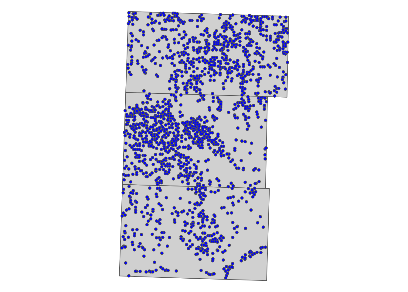

Figure 1.2: Spatial distribution of irrigation wells

---

Here are the rest of the steps we will take to create a regression-ready dataset for our analysis.

1. download groundwater level data observed at USGS monitoring wells from National Water Information System (NWIS) using the dataRetrieval package
2. identify the irrigation wells located within the 2-mile radius of the USGS wells and calculate the total groundwater pumping that occurred around each of the USGS wells by year
3. merge the groundwater pumping data to the groundwater level data

---

Let’s download groundwater level data from NWIS first. The following code downloads groundwater level data for Nebraska from Jan 1, 1990, through Jan 1, 2016.

#--- download groundwater level data ---#
NE_gwl <-
  readNWISdata(
    stateCd = "Nebraska",
    startDate = "1990-01-01",
    endDate = "2016-01-01",
    service = "gwlevels"
  ) %>%
  dplyr::select(site_no, lev_dt, lev_va) %>%
  rename(date = lev_dt, dwt = lev_va)

#--- take a look ---#
head(NE_gwl, 10)

           site_no       date   dwt
1  400008097545301 2000-11-08 17.40
2  400008097545301 2008-10-09 13.99
3  400008097545301 2009-04-09 11.32
4  400008097545301 2009-10-06 15.54
5  400008097545301 2010-04-12 11.15
6  400008100050501 1990-03-15 24.80
7  400008100050501 1990-10-04 27.20
8  400008100050501 1991-03-08 24.20
9  400008100050501 1991-10-07 26.90
10 400008100050501 1992-03-02 24.70

site_no is the unique monitoring well identifier, date is the date of groundwater level monitoring, and dwt is depth to water table.

We calculate the average groundwater level in March by USGS monitoring well (right before the irrigation season starts):¹²

#--- Average depth to water table in March ---#
NE_gwl_march <-
  NE_gwl %>%
  mutate(
    date = as.Date(date),
    month = month(date),
    year = year(date),
  ) %>%
  #--- select observation in March ---#
  filter(year >= 2007, month == 3) %>%
  #--- gwl average in March ---#
  group_by(site_no, year) %>%
  summarize(dwt = mean(dwt))

#--- take a look ---#
head(NE_gwl_march, 10)

# A tibble: 10 × 3
# Groups:   site_no [2]
   site_no          year   dwt
   <chr>           <dbl> <dbl>
 1 400032101022901  2008 118. 
 2 400032101022901  2009 117. 
 3 400032101022901  2010 118. 
 4 400032101022901  2011 118. 
 5 400032101022901  2012 118. 
 6 400032101022901  2013 118. 
 7 400032101022901  2014 116. 
 8 400032101022901  2015 117. 
 9 400038099244601  2007  24.3
10 400038099244601  2008  21.7

Since NE_gwl is missing geographic coordinates for the monitoring wells, we will download them using the readNWISsite() function and select only the monitoring wells that are inside the three counties.

#--- get the list of site ids ---#
NE_site_ls <- NE_gwl$site_no %>% unique()

#--- get the locations of the site ids ---#
sites_info <-
  readNWISsite(siteNumbers = NE_site_ls) %>%
  dplyr::select(site_no, dec_lat_va, dec_long_va) %>%
  #--- turn the data into an sf object ---#
  st_as_sf(coords = c("dec_long_va", "dec_lat_va")) %>%
  #--- NAD 83 ---#
  st_set_crs(4269) %>%
  #--- project to WGS UTM 14 ---#
  st_transform(32614) %>%
  #--- keep only those located inside the three counties ---#
  .[three_counties, ]

---

We now identify irrigation wells that are located within the 2-mile radius of the monitoring wells¹³. We first create polygons of 2-mile radius circles around the monitoring wells (see Figure 1.3).

buffers <- st_buffer(sites_info, dist = 2 * 1609.34) # in meter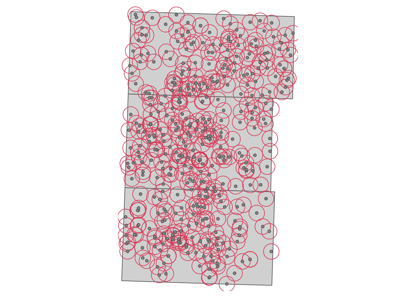

Figure 1.3: 2-mile buffers around USGS monitoring wells

We now identify which irrigation wells are inside each of the buffers and get the associated groundwater pumping values. The st_join() function from the sf package will do the trick.

#--- find irrigation wells inside the buffer and calculate total pumping  ---#
pumping_nearby <- st_join(buffers, urnrd_gw_sf)

Let’s take a look at a USGS monitoring well (site_no = \(400012101323401\)).

filter(pumping_nearby, site_no == 400012101323401, year == 2010)

Simple feature collection with 7 features and 4 fields
Geometry type: POLYGON
Dimension:     XY
Bounding box:  xmin: 279690.7 ymin: 4428006 xmax: 286128 ymax: 4434444
Projected CRS: WGS 84 / UTM zone 14N
             site_no well_id year  vol_af                       geometry
9.3  400012101323401    6331 2010      NA POLYGON ((286128 4431225, 2...
9.24 400012101323401    1883 2010 180.189 POLYGON ((286128 4431225, 2...
9.25 400012101323401    2006 2010  79.201 POLYGON ((286128 4431225, 2...
9.26 400012101323401    2538 2010  68.205 POLYGON ((286128 4431225, 2...
9.27 400012101323401    2834 2010      NA POLYGON ((286128 4431225, 2...
9.28 400012101323401    2834 2010 122.981 POLYGON ((286128 4431225, 2...
9.29 400012101323401    4983 2010      NA POLYGON ((286128 4431225, 2...

As you can see, this well has seven irrigation wells within its 2-mile radius in 2010.

Now, we will get total nearby pumping by monitoring well and year.

(
  total_pumping_nearby <-
    pumping_nearby %>%
    #--- calculate total pumping by monitoring well ---#
    group_by(site_no, year) %>%
    summarize(nearby_pumping = sum(vol_af, na.rm = TRUE)) %>%
    #--- NA means 0 pumping ---#
    mutate(
      nearby_pumping = ifelse(is.na(nearby_pumping), 0, nearby_pumping)
    )
)

Simple feature collection with 2396 features and 3 fields
Geometry type: POLYGON
Dimension:     XY
Bounding box:  xmin: 237904.5 ymin: 4428006 xmax: 313476.5 ymax: 4545687
Projected CRS: WGS 84 / UTM zone 14N
# A tibble: 2,396 × 4
# Groups:   site_no [401]
   site_no          year nearby_pumping                                 geometry
 * <chr>           <int>          <dbl>                            <POLYGON [m]>
 1 400012101323401  2007           571. ((286128 4431225, 286123.6 4431057, 286…
 2 400012101323401  2008           772. ((286128 4431225, 286123.6 4431057, 286…
 3 400012101323401  2009           500. ((286128 4431225, 286123.6 4431057, 286…
 4 400012101323401  2010           451. ((286128 4431225, 286123.6 4431057, 286…
 5 400012101323401  2011           545. ((286128 4431225, 286123.6 4431057, 286…
 6 400012101323401  2012          1028. ((286128 4431225, 286123.6 4431057, 286…
 7 400130101374401  2007           485. ((278847.4 4433844, 278843 4433675, 278…
 8 400130101374401  2008           515. ((278847.4 4433844, 278843 4433675, 278…
 9 400130101374401  2009           351. ((278847.4 4433844, 278843 4433675, 278…
10 400130101374401  2010           374. ((278847.4 4433844, 278843 4433675, 278…
# … with 2,386 more rows

---

We now merge nearby pumping data to the groundwater level data, and transform the data to obtain the dataset ready for regression analysis.

#--- regression-ready data ---#
reg_data <-
  NE_gwl_march %>%
  #--- pick monitoring wells that are inside the three counties ---#
  filter(site_no %in% unique(sites_info$site_no)) %>%
  #--- merge with the nearby pumping data ---#
  left_join(., total_pumping_nearby, by = c("site_no", "year")) %>%
  #--- lead depth to water table ---#
  arrange(site_no, year) %>%
  group_by(site_no) %>%
  mutate(
    #--- lead depth ---#
    dwt_lead1 = dplyr::lead(dwt, n = 1, default = NA, order_by = year),
    #--- first order difference in dwt  ---#
    dwt_dif = dwt_lead1 - dwt
  )

#--- take a look ---#
dplyr::select(reg_data, site_no, year, dwt_dif, nearby_pumping)

# A tibble: 2,022 × 4
# Groups:   site_no [230]
   site_no          year dwt_dif nearby_pumping
   <chr>           <dbl>   <dbl>          <dbl>
 1 400130101374401  2011  NA               358.
 2 400134101483501  2007   2.87           2038.
 3 400134101483501  2008   0.780          2320.
 4 400134101483501  2009  -2.45           2096.
 5 400134101483501  2010   3.97           2432.
 6 400134101483501  2011   1.84           2634.
 7 400134101483501  2012  -1.35            985.
 8 400134101483501  2013  44.8              NA 
 9 400134101483501  2014 -26.7              NA 
10 400134101483501  2015  NA                NA 
# … with 2,012 more rows

---

Finally, we estimate the model using feols() from the fixest package (see here for an introduction).

#--- OLS with site_no and year FEs (error clustered by site_no) ---#
reg_dwt <-
  feols(
    dwt_dif ~ nearby_pumping | site_no + year,
    cluster = "site_no",
    data = reg_data
  )

Here is the regression result.

modelsummary(
  reg_dwt,
  stars = TRUE,
  gof_omit = "IC|Log|Adj|Within|Pseudo"
)

	Model 1
nearby_pumping	0.001***
	(0.000)
Num.Obs.	1342
R2	0.409
Std.Errors	by: site_no
FE: site_no	X
FE: year	X
+ p < 0.1, * p < 0.05, ** p < 0.01, *** p < 0.001

---

---

10. the distance from the surface to the top of the aquifer↩︎

11. For our geographic focus of southwest Nebraska, corn is the dominant crop type. Irrigation for corn happens typically between April through September. For example, this means that changes in groundwater level (\(y_{i,2012} - y_{i,2011}\)) captures the impact of groundwater pumping that occurred April through September in 2011.↩︎

12. month() and year() are from the lubridate package. They extract month and year from a Date object.↩︎

13. This can alternatively be done using the st_is_within_distance() function.↩︎