3.4 Spatial Intersection (cropping join)
Sometimes you face the need to crop spatial objects by polygon boundaries. For example, we found the total length of the railroads inside of each county in Demonstration 4 in Chapter 1.4 by cutting off the parts of the railroads that extend beyond the boundary of counties. Also, we just saw that area-weighted averages cannot be found using st_join() because it does not provide information about how much area of each HUC unit is intersecting with each of its intersecting counties. If we can get the geometry of the intersecting part of the HUC unit and the county, then we can calculate its area, which in turn allows us to find area-weighted averages of joined attributes. For these purposes, we can use sf::st_intersection(). Below, we first illustrate how st_intersection() works for lines-polygons and polygons-polygons intersections (Note that we use the data we generated in Chapter 3.1). Intersections that involve points using st_intersection() is the same as using st_join() because points are length-less and area-less (nothing to cut). Thus, it is not discussed here.
3.4.1 st_intersection()
While st_intersects() returns the indices of intersecting objects, st_intersection() returns intersecting spatial objects with the non-intersecting parts of the sf objects cut out. Moreover, attribute values of the source sf will be merged to its intersecting sfg in the target sf. We will see how it works for lines-polygons and polygons-polygons cases using the toy examples we used to explain how st_intersects() work. Here is the figure of the lines and polygons (Figure 3.22):
ggplot() +
  geom_sf(data = polygons, aes(fill = polygon_name), alpha = 0.3) +
  scale_fill_discrete(name = "Polygons") +
  geom_sf(data = lines, aes(color = line_name)) +
scale_color_discrete(name = "Lines") 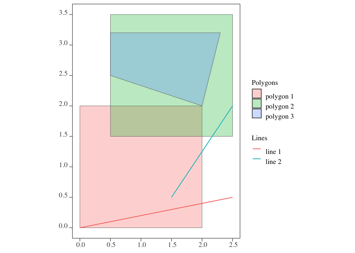
Figure 3.22: Visualization of the points, lines, and polygons
lines and polygons
The following code gets the intersection of the lines and the polygons.
(
intersections_lp <- st_intersection(lines, polygons) %>%
  mutate(int_name = paste0(line_name, "-", polygon_name))
)
Simple feature collection with 3 features and 3 fields
Geometry type: LINESTRING
Dimension: XY
Bounding box: xmin: 0 ymin: 0 xmax: 2.5 ymax: 2
CRS: NA
line_name polygon_name x int_name
1 line 1 polygon 1 LINESTRING (0 0, 2 0.4) line 1-polygon 1
2 line 2 polygon 1 LINESTRING (1.5 0.5, 2 1.25) line 2-polygon 1
2.1 line 2 polygon 2 LINESTRING (2.166667 1.5, 2... line 2-polygon 2As you can see in the output, each instance of the intersections of the lines and polygons become an observation (line 1-polygon 1, line 2-polygon 1, and line 2-polygon 2). The part of the lines that did not intersect with a polygon is cut out and does not remain in the returned sf. To see this, see Figure 3.23 below:
ggplot() +
  #--- here are all the original polygons  ---#
  geom_sf(data = polygons, aes(fill = polygon_name), alpha = 0.3) +
  #--- here is what is returned after st_intersection ---#
  geom_sf(data = intersections_lp, aes(color = int_name), size = 1.5)
Figure 3.23: The outcome of the intersections of the lines and polygons
This further allows us to calculate the length of the part of the lines that are completely contained in polygons, just like we did in Chapter 1.4. Note also that the attribute (polygon_name) of the source sf (the polygons) are merged to their intersecting lines. Therefore, st_intersection() is transforming the original geometries while joining attributes (this is why I call this cropping join).
polygons and polygons
The following code gets the intersection of polygon 1 and polygon 3 with polygon 2.
(
intersections_pp <- st_intersection(polygons[c(1,3), ], polygons[2, ]) %>%
  mutate(int_name = paste0(polygon_name, "-", polygon_name.1))
)
Simple feature collection with 2 features and 3 fields
Geometry type: POLYGON
Dimension: XY
Bounding box: xmin: 0.5 ymin: 1.5 xmax: 2.3 ymax: 3.2
CRS: NA
polygon_name polygon_name.1 x
1 polygon 1 polygon 2 POLYGON ((2 2, 2 1.5, 0.5 1...
3 polygon 3 polygon 2 POLYGON ((0.5 3.2, 2.3 3.2,...
int_name
1 polygon 1-polygon 2
3 polygon 3-polygon 2As you can see in Figure 3.24, each instance of the intersections of polygons 1 and 3 against polygon 2 becomes an observation (polygon 1-polygon 2 and polygon 3-polygon 2). Just like the lines-polygons case, the non-intersecting part of polygons 1 and 3 are cut out and do not remain in the returned sf. We will see later that st_intersection() can be used to find area-weighted values from the intersecting polygons with help from st_area().
ggplot() +
  #--- here are all the original polygons  ---#
  geom_sf(data = polygons, aes(fill = polygon_name), alpha = 0.3) +
  #--- here is what is returned after st_intersection ---#
  geom_sf(data = intersections_pp, aes(fill = int_name))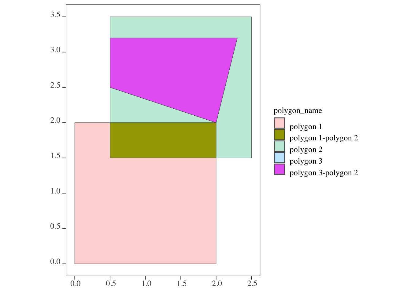
Figure 3.24: The outcome of the intersections of polygon 2 and polygons 1 and 3
3.4.2 Area-weighted average
Let’s now get back to the example of HUC units and county-level corn acres data we saw in Chapter 3.3. We would like to find area-weighted average of corn acres instead of the simple average of corn acres.
Using st_intersection(), for each of the HUC polygons, we find the intersecting counties, and then divide it into parts based on the boundary of the intersecting polygons.
(
HUC_intersections <- st_intersection(HUC_IA, IA_corn) %>%
  mutate(huc_county = paste0(HUC_CODE, "-", county_code))
)
Simple feature collection with 349 features and 5 fields
Geometry type: GEOMETRY
Dimension: XY
Bounding box: xmin: 203228.6 ymin: 4470941 xmax: 736832.9 ymax: 4822687
Projected CRS: NAD83 / UTM zone 15N
First 10 features:
HUC_CODE county_code year acres geometry
732 07080207 083 2018 183500 POLYGON ((482923.9 4711643,...
803 07080205 083 2018 183500 POLYGON ((499725.6 4696873,...
826 07080105 083 2018 183500 POLYGON ((461853.2 4682925,...
627 10170204 141 2018 167000 POLYGON ((269364.9 4793311,...
687 10230003 141 2018 167000 POLYGON ((271504.3 4754685,...
731 10230002 141 2018 167000 POLYGON ((267684.6 4790972,...
683 07100003 081 2018 184500 POLYGON ((435951.2 4789348,...
686 07080203 081 2018 184500 MULTIPOLYGON (((459303.2 47...
732.1 07080207 081 2018 184500 POLYGON ((429573.1 4779788,...
747 07100005 081 2018 184500 POLYGON ((421044.8 4772268,...
huc_county
732 07080207-083
803 07080205-083
826 07080105-083
627 10170204-141
687 10230003-141
731 10230002-141
683 07100003-081
686 07080203-081
732.1 07080207-081
747 07100005-081The key difference from the st_join() example is that each observation of the returned data is a unique HUC-county intersection. Figure 3.25 below is a map of all the intersections of the HUC unit with HUC_CODE ==10170203 and the four intersecting counties.
tm_shape(filter(HUC_intersections, HUC_CODE == "10170203")) +
  tm_polygons(col = "huc_county") +
  tm_layout(frame = FALSE)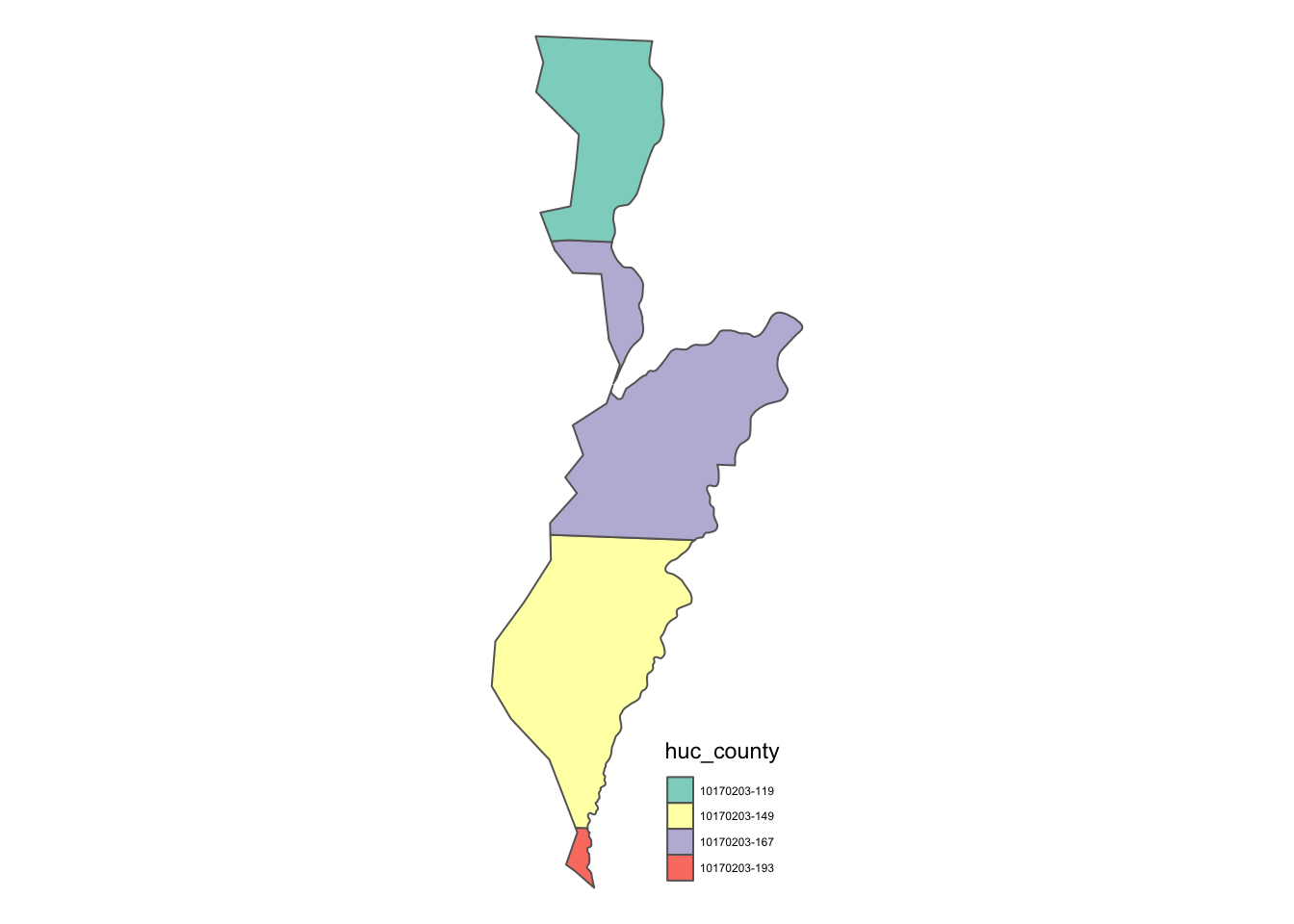
Figure 3.25: Intersections of a HUC unit and Iowa counties
Note also that the attributes of county data are joined as you can see acres in the output above. As I said earlier, st_intersection() is a spatial kind of spatial join where the resulting observations are the intersections of the target and source sf objects.
In order to find the area-weighted average of corn acres, you can use st_area() first to calculate the area of the intersections, and then find the area-weighted average as follows:
(
HUC_aw_acres <- HUC_intersections %>%
  #--- get area ---#
  mutate(area = as.numeric(st_area(.))) %>%
  #--- get area-weight by HUC unit ---#
  group_by(HUC_CODE) %>%
  mutate(weight = area / sum(area)) %>%
  #--- calculate area-weighted corn acreage by HUC unit ---#
  summarize(aw_acres = sum(weight * acres))
)
Simple feature collection with 55 features and 2 fields
Geometry type: GEOMETRY
Dimension: XY
Bounding box: xmin: 203228.6 ymin: 4470941 xmax: 736832.9 ymax: 4822687
Projected CRS: NAD83 / UTM zone 15N
# A tibble: 55 × 3
HUC_CODE aw_acres geometry
<chr> <dbl> <GEOMETRY [m]>
1 07020009 251185. POLYGON ((421060.3 4797550, 420940.3 4797420, 420860.3 479…
2 07040008 165000 POLYGON ((602922.4 4817166, 602862.4 4816996, 602772.4 481…
3 07060001 105234. MULTIPOLYGON (((649333.8 4761761, 648933.7 4761621, 648793…
4 07060002 140201. MULTIPOLYGON (((593780.7 4816946, 594000.7 4816865, 594380…
5 07060003 149000 MULTIPOLYGON (((692011.6 4712966, 691981.6 4712956, 691881…
6 07060004 162123. POLYGON ((652046.5 4718813, 651916.4 4718783, 651786.4 471…
7 07060005 142428. POLYGON ((734140.4 4642126, 733620.4 4641926, 733520.3 464…
8 07060006 159635. POLYGON ((720485.9 4656371, 720355.8 4656291, 720275.8 465…
9 07080101 115572. POLYGON ((666760.8 4558401, 666630.9 4558362, 666510.8 455…
10 07080102 160008. POLYGON ((635896.1 4675834, 636036.2 4675844, 636316.3 467…
# … with 45 more rows