5.2 Extracting Values from Raster Layers for Vector Data
In this section, we will learn how to extract information from raster layers for spatial units represented as vector data (points and polygons). For the demonstrations in this section, we use the following datasets:
- Raster: PRISM tmax data cropped to Kansas state border for 07/01/2018 (obtained in 5.1) and 07/02/2018 (downloaded below)
- Polygons: Kansas county boundaries (obtained in 5.1)
- Points: Irrigation wells in Kansas (imported below)
5.2.1 Simple visual illustrations of raster data extraction
Extracting to Points
Figure 5.4 shows visually what we mean by “extract raster values to points.”
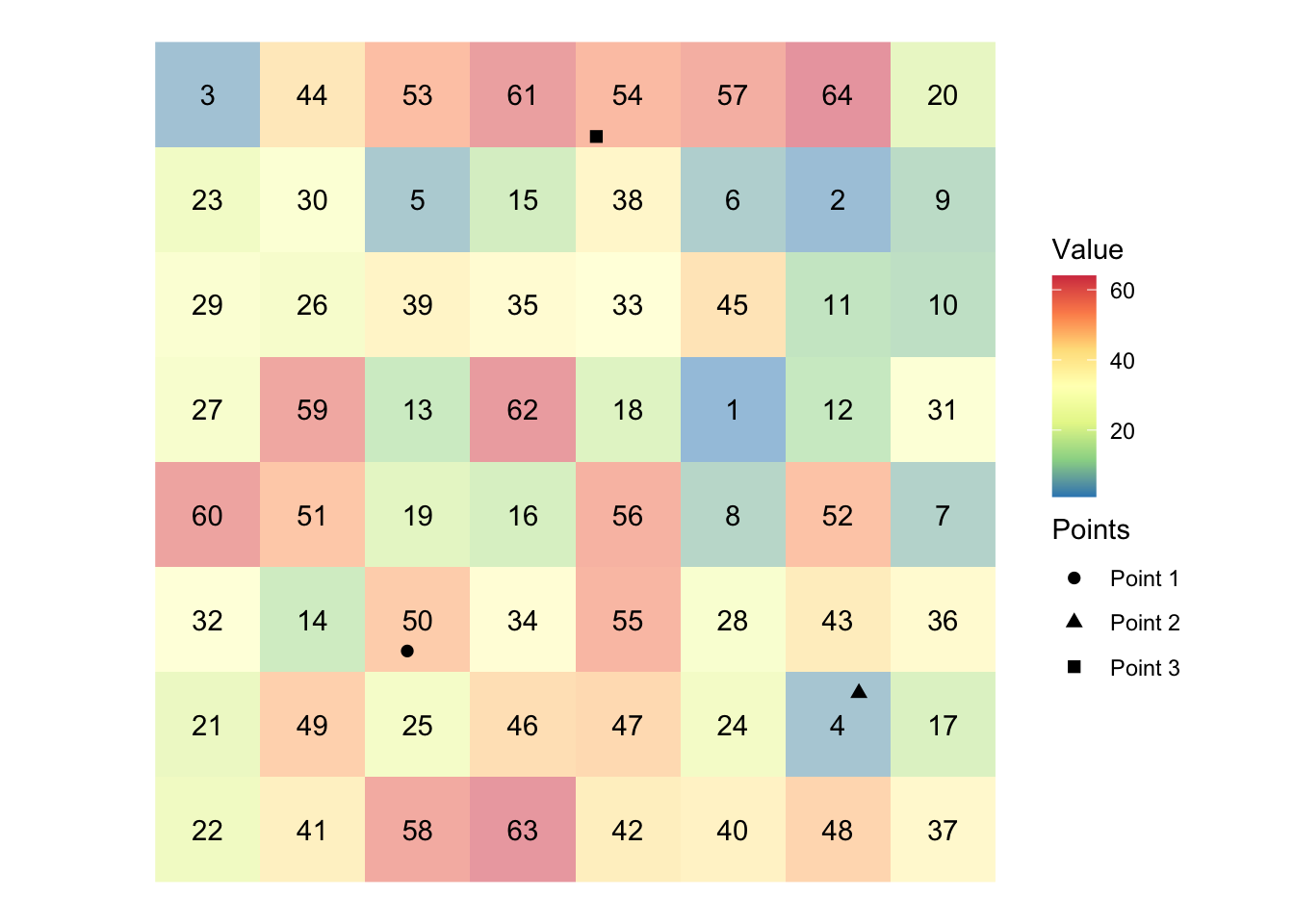
Figure 5.4: Visual illustration of raster data extraction for points data
In the figure, we have grids (cells) and each grid holds a value (presented at the center). There are three points. We will find which grid the points fall inside and get the associated values and assign them to the points. In this example, Points 1, 2, and 3 will have 50, 4, 54, respectively,
Extracting to Polygons
Figure 5.5 shows visually what we mean by “extract raster values to polygons.”
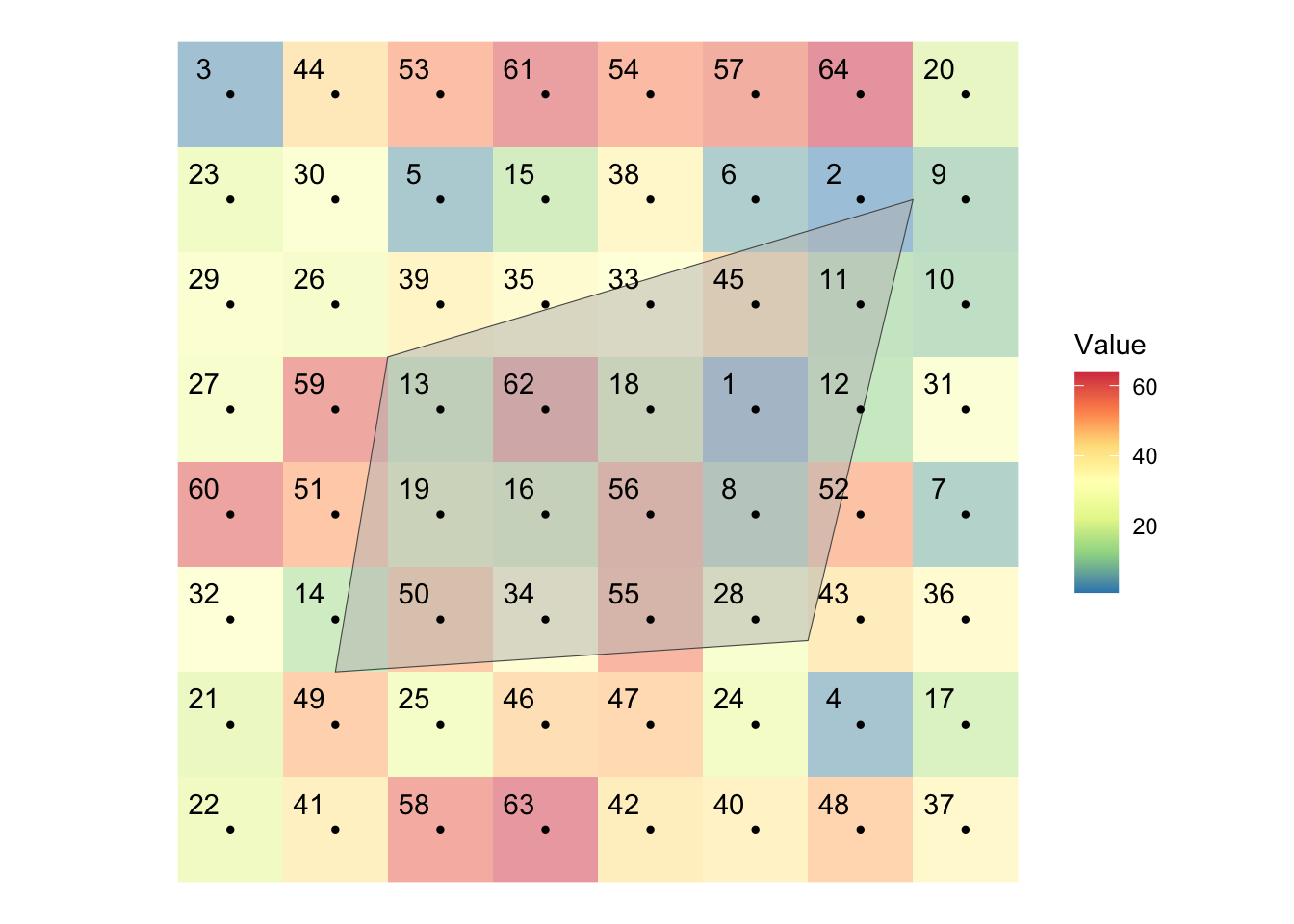
Figure 5.5: Visual illustration of raster data extraction for polygons data
There is a polygon overlaid on top of the cells along with their centroids represented by black dots. Extracting raster values to a polygon means finding raster cells that intersect with the polygons and get the value of all those cells and assigns them to the polygon. As you can see some cells are completely inside the polygon, while others are only partially overlapping with the polygon. Depending on the function you use and its options, you regard different cells as being spatially related to the polygons. For example, by default, terra::extract() will extract only the cells whose centroid is inside the polygon. But, you can add an option to include the cells that are only partially intersected with the polygon. In such a case, you can also get the fraction of the cell what is overlapped with the polygon, which enables us to find area-weighted values later. We will discuss the details these below.
PRISM tmax data for 07/02/2018
#--- download PRISM precipitation data ---#
get_prism_dailys(
  type = "tmax",
  date = "2018-07-02",
  keepZip = FALSE
)

#--- the file name of the PRISM data just downloaded ---#
prism_file <- "Data/PRISM_tmax_stable_4kmD2_20180702_bil/PRISM_tmax_stable_4kmD2_20180702_bil.bil"

#--- read in the prism data and crop it to Kansas state border ---#
prism_tmax_0702_KS_sr <- rast(prism_file) %>%
  terra::crop(KS_county_sf)
Irrigation wells in Kansas:
#--- read in the KS points data ---#
(
KS_wells <- readRDS("Data/Chap_5_wells_KS.rds")
)
Simple feature collection with 37647 features and 1 field
Geometry type: POINT
Dimension: XY
Bounding box: xmin: -102.0495 ymin: 36.99552 xmax: -94.62089 ymax: 40.00199
Geodetic CRS: NAD83
First 10 features:
well_id geometry
1 1 POINT (-100.4423 37.52046)
2 3 POINT (-100.7118 39.91526)
3 5 POINT (-99.15168 38.48849)
4 7 POINT (-101.8995 38.78077)
5 8 POINT (-100.7122 38.0731)
6 9 POINT (-97.70265 39.04055)
7 11 POINT (-101.7114 39.55035)
8 12 POINT (-95.97031 39.16121)
9 15 POINT (-98.30759 38.26787)
10 17 POINT (-100.2785 37.71539)Here is how the wells are spatially distributed over the PRISM grids and Kansas county borders (Figure 5.6):
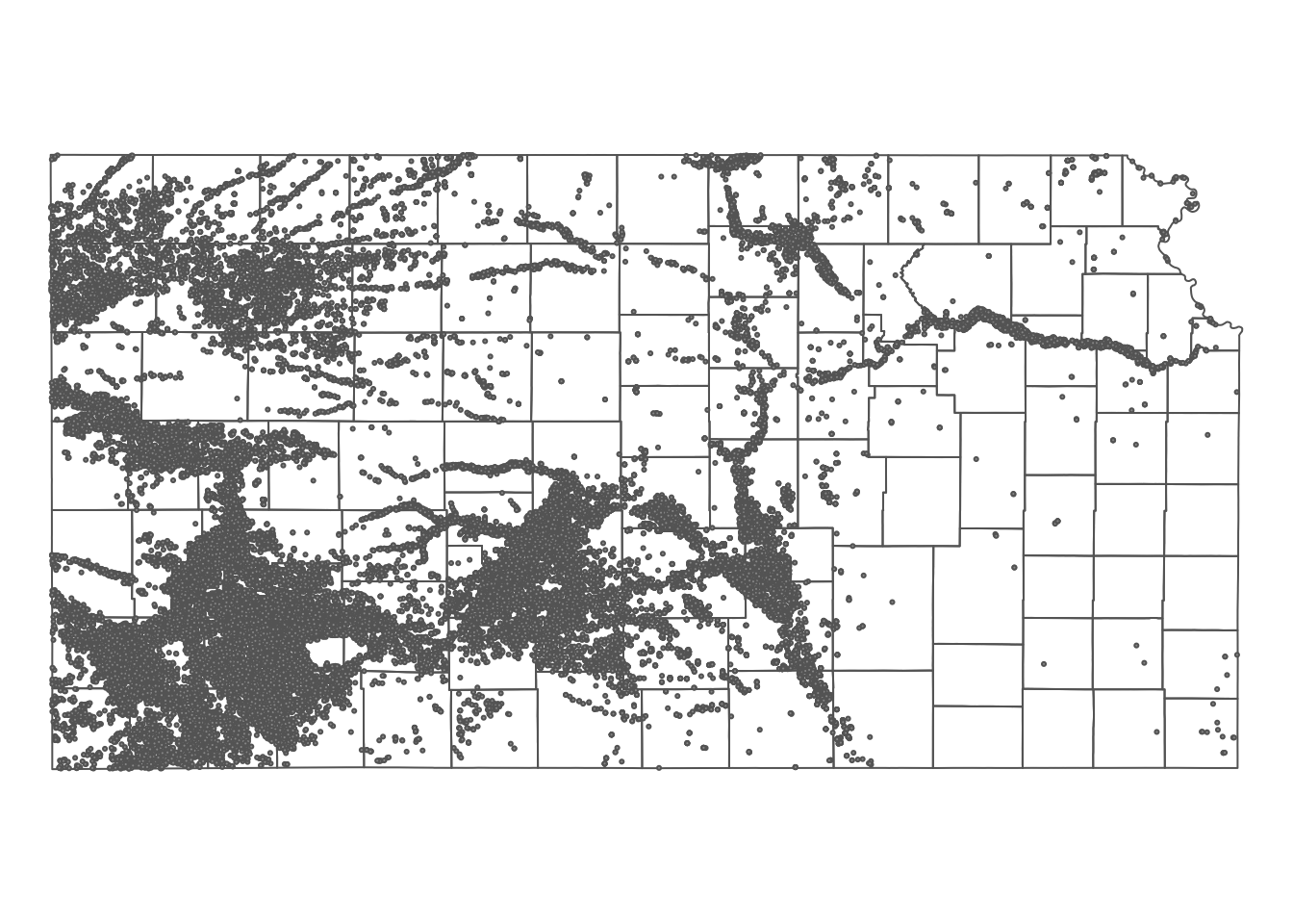
Figure 5.6: Map of Kansas county borders, irrigation wells, and PRISM tmax
5.2.2 Extracting to Points
You can extract values from raster layers to points using terra::extract(). terra::extract() finds which raster cell each of the points is located within and assigns the value of the cell to the point.
#--- syntax (this does not run) ---#
terra::extract(raster, points)
Let’s extract tmax values from the PRISM tmax layer (prism_tmax_0701_KS_sr) to the irrigation wells:
tmax_from_prism <- terra::extract(prism_tmax_0701_KS_sr, KS_wells)Error in (function (classes, fdef, mtable) : unable to find an inherited method for function 'extract' for signature '"SpatRaster", "sf"'Oh, okay. So, the problem is that the points data (KS_wells) is an sf object, and terra::extract() does not like it (I thought this would be fixed by now …). Let’s turn KS_wells into an SpatVect object and then apply terra::extract():
tmax_from_prism <- terra::extract(prism_tmax_0701_KS_sr, vect(KS_wells))

#--- take a look ---#
head(tmax_from_prism)
ID PRISM_tmax_stable_4kmD2_20180701_bil
1 1 34.241
2 2 29.288
3 3 32.585
4 4 30.104
5 5 34.232
6 6 35.168The resulting object is a data.frame, where the ID variable represents the order of the observations in the points data and the second column represents that values extracted for the points from the raster cells. So, you can assign the extracted values as a new variable of the points data as follows:
KS_wells$tmax_07_01 <- tmax_from_prism[, -1]Extracting values from a multi-layer SpatRaster works the same way. Here, we combine prism_tmax_0701_KS_sr and prism_tmax_0702_KS_sr to create a multi-layer SpatRaster and then extract values from them.
#--- create a multi-layer SpatRaster ---#
prism_tmax_stack <- c(prism_tmax_0701_KS_sr, prism_tmax_0702_KS_sr)

#--- extract tmax values ---#
tmax_from_prism_stack <- terra::extract(prism_tmax_stack, vect(KS_wells))

#--- take a look ---#
head(tmax_from_prism_stack)
ID PRISM_tmax_stable_4kmD2_20180701_bil PRISM_tmax_stable_4kmD2_20180702_bil
1 1 34.241 30.544
2 2 29.288 29.569
3 3 32.585 29.866
4 4 30.104 29.819
5 5 34.232 30.481
6 6 35.168 30.640We now have two columns that hold values extracted from the raster cells: the 2nd column for the 1st raster layer and the 3rd column for the 2nd raster layer in prism_tmax_stack.
Side note:
Interestingly, terra::extract() can work with sf as long as the raster object is of type Raster\(^*\). In the code below, prism_tmax_stack is converted to RasterStack before terra::extract() does its job and it works just fine.
tmax_from_prism <- terra::extract(as(prism_tmax_stack, "Raster"), KS_wells)#--- take a look ---#
head(tmax_from_prism) ID PRISM_tmax_stable_4kmD2_20180701_bil
1 1 34.241
2 2 29.288
3 3 32.585
4 4 30.104
5 5 34.232
6 6 35.168#--- check the class ---#
class(tmax_from_prism)[1] "data.frame"As you can see, the resulting object is a matrix instead of a data.frame. Now, let’s see if we can use a SpatVect instead of an sf.
tmax_from_prism <-
  terra::extract(
    as(prism_tmax_stack, "Raster"),
    vect(KS_wells)
  )
Error in (function (classes, fdef, mtable) : unable to find an inherited method for function 'extract' for signature '"RasterBrick", "SpatVector"'So, it does not work. It turns out that terra::extract() works for the combinations of SpatRaster-SpatVect or Raster\(^*\)-sf/sp.
5.2.3 Extracting to Polygons (terra way)
You can use terra::extract() for extracting raster cell values for polygons as well. For each of the polygons, it will identify all the raster cells whose center lies inside the polygon and assign the vector of values of the cells to the polygon. Let’s first convert KS_county_sf (an sf object) to a SpatVector.
#--- Kansas boundary (SpatVector) ---#
KS_county_sv <- vect(KS_county_sf)
Now, let’s extract tmax values for each of the KS counties.
#--- extract values from the raster for each county ---#
tmax_by_county <- terra::extract(prism_tmax_0701_KS_sr, KS_county_sv)
#--- check the class ---#
class(tmax_by_county)[1] "data.frame"#--- take a look ---#
head(tmax_by_county) ID PRISM_tmax_stable_4kmD2_20180701_bil
1 1 34.228
2 1 34.222
3 1 34.256
4 1 34.268
5 1 34.262
6 1 34.477#--- take a look ---#
tail(tmax_by_county) ID PRISM_tmax_stable_4kmD2_20180701_bil
12840 105 34.185
12841 105 34.180
12842 105 34.241
12843 105 34.381
12844 105 34.295
12845 105 34.267So, terra::extract() returns a data.frame, where ID values represent the corresponding row number in the polygons data. For example, the observations with ID == n are for the nth polygon. Using this information, you can easily merge the extraction results to the polygons data. Suppose you are interested in the mean of the tmax values of the intersecting cells for each of the polygons, then you can do the following:
#--- get mean tmax ---#
mean_tmax <-
  tmax_by_county %>%
  group_by(ID) %>%
  summarize(tmax = mean(PRISM_tmax_stable_4kmD2_20180701_bil))

(
KS_county_sf <-
  #--- back to sf ---#
  st_as_sf(KS_county_sv) %>%
  #--- define ID ---#
  mutate(ID := seq_len(nrow(.))) %>%
  #--- merge by ID ---#
  left_join(., mean_tmax, by = "ID")
)
Simple feature collection with 105 features and 14 fields
Geometry type: POLYGON
Dimension: XY
Bounding box: xmin: -102.0517 ymin: 36.99302 xmax: -94.58841 ymax: 40.00316
Geodetic CRS: NAD83
First 10 features:
STATEFP COUNTYFP COUNTYNS AFFGEOID GEOID NAME
1 20 075 00485327 0500000US20075 20075 Hamilton
2 20 149 00485038 0500000US20149 20149 Pottawatomie
3 20 003 00484971 0500000US20003 20003 Anderson
4 20 033 00484986 0500000US20033 20033 Comanche
5 20 189 00485056 0500000US20189 20189 Stevens
6 20 161 00485044 0500000US20161 20161 Riley
7 20 025 00484982 0500000US20025 20025 Clark
8 20 163 00485045 0500000US20163 20163 Rooks
9 20 091 00485010 0500000US20091 20091 Johnson
10 20 187 00485055 0500000US20187 20187 Stanton
NAMELSAD STUSPS STATE_NAME LSAD ALAND AWATER ID tmax
1 Hamilton County KS Kansas 06 2580958328 2893322 1 34.21421
2 Pottawatomie County KS Kansas 06 2177507162 54149295 2 32.58354
3 Anderson County KS Kansas 06 1501263686 10599981 3 34.63195
4 Comanche County KS Kansas 06 2041681089 3604155 4 33.40829
5 Stevens County KS Kansas 06 1883593926 464936 5 34.01768
6 Riley County KS Kansas 06 1579116499 32002514 6 35.54426
7 Clark County KS Kansas 06 2524300310 6603384 7 34.47948
8 Rooks County KS Kansas 06 2306454194 11962259 8 33.55797
9 Johnson County KS Kansas 06 1226694710 16303985 9 34.77049
10 Stanton County KS Kansas 06 1762103387 178555 10 33.56413
geometry
1 POLYGON ((-102.0446 38.0480...
2 POLYGON ((-96.72833 39.4271...
3 POLYGON ((-95.51879 38.0671...
4 POLYGON ((-99.54467 37.3047...
5 POLYGON ((-101.5566 37.3884...
6 POLYGON ((-96.96095 39.2867...
7 POLYGON ((-100.1072 37.4748...
8 POLYGON ((-99.60527 39.2638...
9 POLYGON ((-95.05647 38.9660...
10 POLYGON ((-102.0419 37.5411...Instead of finding the mean after applying terra::extract() as done above, you can do that within terra::extract() using the fun option.
#--- extract values from the raster for each county ---#
tmax_by_county <-
  terra::extract(
    prism_tmax_0701_KS_sr,
    KS_county_sv,
    fun = mean
  )
#--- take a look ---#
head(tmax_by_county) ID PRISM_tmax_stable_4kmD2_20180701_bil
1 1 34.21421
2 2 32.58354
3 3 34.63195
4 4 33.40829
5 5 34.01768
6 6 35.54426You can apply other summary functions like min(), max(), sum().
Extracting values from a multi-layer raster data works exactly the same way except that data processing after the value extraction is slightly more complicated.
#--- extract from a multi-layer raster object ---#
tmax_by_county_from_stack <-
  terra::extract(
    prism_tmax_stack,
    KS_county_sv
  )

#--- take a look ---#
head(tmax_by_county_from_stack)
ID PRISM_tmax_stable_4kmD2_20180701_bil PRISM_tmax_stable_4kmD2_20180702_bil
1 1 31.457 29.864
2 1 31.503 29.927
3 1 31.604 29.966
4 1 31.718 30.009
5 1 31.741 30.079
6 1 31.881 30.128Similar to the single-layer case, the resulting object is a data.frame and you have two columns corresponding to each of the layers in the two-layer raster object.
Sometimes, you would like to have how much of the raster cells are intersecting with the intersecting polygon to find area-weighted summary later. In that case, you can add exact = TRUE option to terra::extract().
#--- extract from a multi-layer raster object ---#
tmax_by_county_from_stack <-
  terra::extract(
    prism_tmax_stack,
    KS_county_sv,
    exact = TRUE
  )

#--- take a look ---#
head(tmax_by_county_from_stack)
ID PRISM_tmax_stable_4kmD2_20180701_bil PRISM_tmax_stable_4kmD2_20180702_bil
1 1 31.457 29.864
2 1 31.503 29.927
3 1 31.604 29.966
4 1 31.718 30.009
5 1 31.741 30.079
6 1 31.881 30.128
fraction
1 0.4514711
2 0.7977501
3 0.7975878
4 0.7974255
5 0.7972632
6 0.7971788As you can see, now you have fraction column to the resulting data.frame and you can find area-weighted summary of the extracted values like this:
tmax_by_county_from_stack %>%
  group_by(ID) %>%
  summarize(
    tmax_0701 = sum(fraction * PRISM_tmax_stable_4kmD2_20180701_bil) / sum(fraction),
    tmax_0702 = sum(fraction * PRISM_tmax_stable_4kmD2_20180702_bil) / sum(fraction)
  )
# A tibble: 105 × 3
ID tmax_0701 tmax_0702
<dbl> <dbl> <dbl>
1 1 32.3 30.1
2 2 35.7 28.8
3 3 34.9 29.4
4 4 33.8 29.9
5 5 34.1 30.5
6 6 35.6 29.8
7 7 34.1 31.0
8 8 33.0 28.9
9 9 35.1 29.7
10 10 33.3 30.2
# … with 95 more rows5.2.4 Extracting to Polygons (exactextractr way)
exact_extract() function from the exactextractr package is a faster alternative than terra::extract() for a large raster data as we confirm later (exact_extract() does not work with points data at the moment).74 exact_extract() also provides a coverage fraction value for each of the cell-polygon intersections. The syntax of exact_extract() is very much similar to terra::extract().
#--- syntax (this does not run) ---#
exact_extract(raster, polygons)
exact_extract() can accept both SpatRaster and Raster\(^*\) objects as the raster object. However, while it accepts sf as the polygons object, but it does not accept SpatVect.
Let’s get tmax values from the PRISM raster layer for Kansas county polygons, the following does the job:
library("exactextractr")

#--- extract values from the raster for each county ---#
tmax_by_county <-
  exact_extract(
    prism_tmax_0701_KS_sr,
    KS_county_sf,
    #--- this is for not displaying progress bar ---#
    progress = FALSE
  )
The resulting object is a list of data.frames where ith element of the list is for ith polygon of the polygons sf object.
#--- take a look at the first 6 rows of the first two list elements ---#
tmax_by_county[1:2] %>% lapply(function(x) head(x))
[[1]]
value coverage_fraction
1 31.457 0.4514454
2 31.503 0.7977046
3 31.604 0.7975423
4 31.718 0.7973800
5 31.741 0.7972176
6 31.881 0.7971521
[[2]]
value coverage_fraction
1 35.492 0.04248790
2 35.552 0.08910853
3 35.638 0.08570296
4 35.668 0.08580886
5 35.655 0.08667702
6 35.543 0.08706726For each element of the list, you see value and coverage_fraction. value is the tmax value of the intersecting raster cells, and coverage_fraction is the fraction of the intersecting area relative to the full raster grid, which can help find coverage-weighted summary of the extracted values (like fraction variable when you use terra::extract() with exact = TRUE).
We can take advantage of dplyr::bind_rows() to combine the list of the datasets into a single data.frame. In doing so, you can use .id option to create a new identifier column that links each row to its original data.
(
#--- combine ---#
tmax_combined <- bind_rows(tmax_by_county, .id = "id") %>%
  as_tibble()
)
# A tibble: 15,149 × 3
id value coverage_fraction
<chr> <dbl> <dbl>
1 1 31.5 0.451
2 1 31.5 0.798
3 1 31.6 0.798
4 1 31.7 0.797
5 1 31.7 0.797
6 1 31.9 0.797
7 1 31.9 0.799
8 1 32.0 0.801
9 1 32.0 0.804
10 1 32.0 0.807
# … with 15,139 more rowsdata.table users can use rbindlist() with the idcol option like below:
rbindlist(tmax_by_county, idcol = "id") id value coverage_fraction
1: 1 31.457 0.4514454
2: 1 31.503 0.7977046
3: 1 31.604 0.7975423
4: 1 31.718 0.7973800
5: 1 31.741 0.7972176
---
15145: 105 33.653 0.2876675
15146: 105 33.670 0.2943960
15147: 105 33.737 0.3016187
15148: 105 33.789 0.3093757
15149: 105 33.817 0.1121131Note that id value of i represents ith element of the list, which in turn corresponds to ith polygon in the polygons sf data. Let’s summarize the data by id and then merge it back to the polygons sf data. Here, we calculate coverage-weighted mean of tmax.
#--- weighted mean ---#
(
tmax_by_id <- tmax_combined %>%
  #--- convert from character to numeric  ---#
  mutate(id = as.numeric(id)) %>%
  #--- group summary ---#
  group_by(id) %>%
  summarise(tmax_aw = sum(value * coverage_fraction) / sum(coverage_fraction))
)
# A tibble: 105 × 2
id tmax_aw
<dbl> <dbl>
1 1 32.3
2 2 35.7
3 3 34.9
4 4 33.8
5 5 34.1
6 6 35.6
7 7 34.1
8 8 33.0
9 9 35.1
10 10 33.3
# … with 95 more rows#--- merge ---#
KS_county_sf %>%
mutate(id := seq_len(nrow(.))) %>%
left_join(., tmax_by_id, by = "id") %>%
dplyr::select(id, tmax_aw)Simple feature collection with 105 features and 2 fields
Geometry type: POLYGON
Dimension: XY
Bounding box: xmin: -102.0517 ymin: 36.99302 xmax: -94.58841 ymax: 40.00316
Geodetic CRS: NAD83
First 10 features:
id tmax_aw geometry
1 1 32.31343 POLYGON ((-102.0446 38.0480...
2 2 35.67419 POLYGON ((-96.72833 39.4271...
3 3 34.89472 POLYGON ((-95.51879 38.0671...
4 4 33.81025 POLYGON ((-99.54467 37.3047...
5 5 34.08601 POLYGON ((-101.5566 37.3884...
6 6 35.57546 POLYGON ((-96.96095 39.2867...
7 7 34.05798 POLYGON ((-100.1072 37.4748...
8 8 33.02438 POLYGON ((-99.60527 39.2638...
9 9 35.11876 POLYGON ((-95.05647 38.9660...
10 10 33.32522 POLYGON ((-102.0419 37.5411...Extracting values from RasterStack works in exactly the same manner as RasterLayer.
tmax_by_county_stack <-
  exact_extract(
    prism_tmax_stack,
    KS_county_sf,
    progress = F
  )

#--- take a look at the first 6 lines of the first element---#
tmax_by_county_stack[[1]] %>% head()
PRISM_tmax_stable_4kmD2_20180701_bil PRISM_tmax_stable_4kmD2_20180702_bil
1 34.235 29.632
2 34.228 29.562
3 34.222 29.557
4 34.256 29.662
5 34.268 29.704
6 34.262 29.750
coverage_fraction
1 0.0007206142
2 0.7114530802
3 0.7162888646
4 0.7163895965
5 0.7166024446
6 0.7175790071As you can see above, exact_extract() appends additional columns for additional layers.
#--- combine them ---#
tmax_all_combined <- bind_rows(tmax_by_county_stack, .id = "id")

#--- take a look ---#
head(tmax_all_combined)
id PRISM_tmax_stable_4kmD2_20180701_bil PRISM_tmax_stable_4kmD2_20180702_bil
1 1 34.235 29.632
2 1 34.228 29.562
3 1 34.222 29.557
4 1 34.256 29.662
5 1 34.268 29.704
6 1 34.262 29.750
coverage_fraction
1 0.0007206142
2 0.7114530802
3 0.7162888646
4 0.7163895965
5 0.7166024446
6 0.7175790071In order to find the coverage-weighted tmax by date, you can first pivot it to a long format using dplyr::pivot_longer().
#--- pivot to a longer format ---#
(
tmax_long <- pivot_longer(
  tmax_all_combined,
  -c(id, coverage_fraction),
  names_to = "date",
  values_to = "tmax"
  )
)
# A tibble: 30,298 × 4
id coverage_fraction date tmax
<chr> <dbl> <chr> <dbl>
1 1 0.000721 PRISM_tmax_stable_4kmD2_20180701_bil 34.2
2 1 0.000721 PRISM_tmax_stable_4kmD2_20180702_bil 29.6
3 1 0.711 PRISM_tmax_stable_4kmD2_20180701_bil 34.2
4 1 0.711 PRISM_tmax_stable_4kmD2_20180702_bil 29.6
5 1 0.716 PRISM_tmax_stable_4kmD2_20180701_bil 34.2
6 1 0.716 PRISM_tmax_stable_4kmD2_20180702_bil 29.6
7 1 0.716 PRISM_tmax_stable_4kmD2_20180701_bil 34.3
8 1 0.716 PRISM_tmax_stable_4kmD2_20180702_bil 29.7
9 1 0.717 PRISM_tmax_stable_4kmD2_20180701_bil 34.3
10 1 0.717 PRISM_tmax_stable_4kmD2_20180702_bil 29.7
# … with 30,288 more rowsAnd then find coverage-weighted tmax by date:
(
tmax_long %>%
  group_by(id, date) %>%
  summarize(tmax = sum(tmax * coverage_fraction) / sum(coverage_fraction))
)
# A tibble: 210 × 3
# Groups: id [105]
id date tmax
<chr> <chr> <dbl>
1 1 PRISM_tmax_stable_4kmD2_20180701_bil 34.2
2 1 PRISM_tmax_stable_4kmD2_20180702_bil 29.7
3 10 PRISM_tmax_stable_4kmD2_20180701_bil 33.6
4 10 PRISM_tmax_stable_4kmD2_20180702_bil 31.2
5 100 PRISM_tmax_stable_4kmD2_20180701_bil 35.2
6 100 PRISM_tmax_stable_4kmD2_20180702_bil 29.8
7 101 PRISM_tmax_stable_4kmD2_20180701_bil 29.9
8 101 PRISM_tmax_stable_4kmD2_20180702_bil 30.0
9 102 PRISM_tmax_stable_4kmD2_20180701_bil 33.3
10 102 PRISM_tmax_stable_4kmD2_20180702_bil 30.2
# … with 200 more rowsFor data.table users, this does the same:
(
tmax_all_combined %>%
  data.table() %>%
  melt(id.var = c("id", "coverage_fraction")) %>%
  .[, .(tmax = sum(value * coverage_fraction) / sum(coverage_fraction)), by = .(id, variable)]
)
id variable tmax
1: 1 PRISM_tmax_stable_4kmD2_20180701_bil 34.21148
2: 2 PRISM_tmax_stable_4kmD2_20180701_bil 32.59907
3: 3 PRISM_tmax_stable_4kmD2_20180701_bil 34.62680
4: 4 PRISM_tmax_stable_4kmD2_20180701_bil 33.41405
5: 5 PRISM_tmax_stable_4kmD2_20180701_bil 34.02482
---
206: 101 PRISM_tmax_stable_4kmD2_20180702_bil 30.01027
207: 102 PRISM_tmax_stable_4kmD2_20180702_bil 30.23891
208: 103 PRISM_tmax_stable_4kmD2_20180702_bil 30.16537
209: 104 PRISM_tmax_stable_4kmD2_20180702_bil 30.54567
210: 105 PRISM_tmax_stable_4kmD2_20180702_bil 30.85847