8.3 Color scale

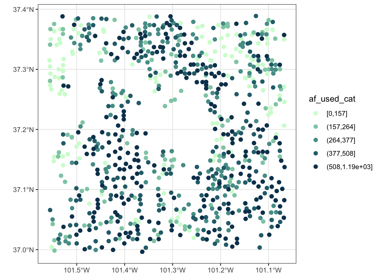
Color scale refers to the way variable values are mapped to colors on a figure. For example, in the example below, the color scale for fill maps the value of af_used to a gradient of colors: dark blue for low values to light blue for high values of af_used.

tmax_long_df <- readRDS("Data/tmax_Jan_09_stars.rds") %>%
  as.data.frame(xy = TRUE) %>%
  na.omit()

g_col_scale <- ggplot() +
  geom_raster(data = tmax_long_df, aes(x = x, y = y, fill = tmax)) +
  facet_wrap(date ~ .) +
  coord_equal() +
  theme_void() +
  theme(
    legend.position = "bottom"
  )

Often times, it is aesthetically desirable to change the default color scale of ggplot2. For example, if you would like to color-differentiate temperature values, you might want to start from blue for low values to red for high values.

You can control the color scale using scale_*() functions. Which scale_*() function to use depends on the type of aesthetics (fill or color) and whether the aesthetic variable is continuous or discrete. Providing a wrong kind of scale_*() function results in an error.

8.3.1 Viridis color maps

The ggplot2 packages offers scale_A_viridis_B() functions for viridis color map, where A is the type of aesthetics attribute (fill, color), and B is the type of variable. For example, scale_fill_viridis_c() can be used for fill aesthetics applied to a continuous variable.

There are five types of palettes available under the viridis color map and can be selected using the option = option. Here is a visualization of all the five palettes.

data("geyser", package = "MASS")

ggplot(geyser, aes(x = duration, y = waiting)) +
  xlim(0.5, 6) +
  ylim(40, 110) +
  stat_density2d(aes(fill = ..level..), geom = "polygon") +
  theme_bw() +
  theme(panel.grid = element_blank()) -> gg

(gg + scale_fill_viridis_c(option = "A") + labs(x = "magma", y = NULL)) /
  (gg + scale_fill_viridis_c(option = "B") + labs(x = "inferno", y = NULL)) /
  (gg + scale_fill_viridis_c(option = "C") + labs(x = "plasma", y = NULL)) /
  (gg + scale_fill_viridis_c(option = "D") + labs(x = "viridis", y = NULL)) /
  (gg + scale_fill_viridis_c(option = "E") + labs(x = "cividis", y = NULL))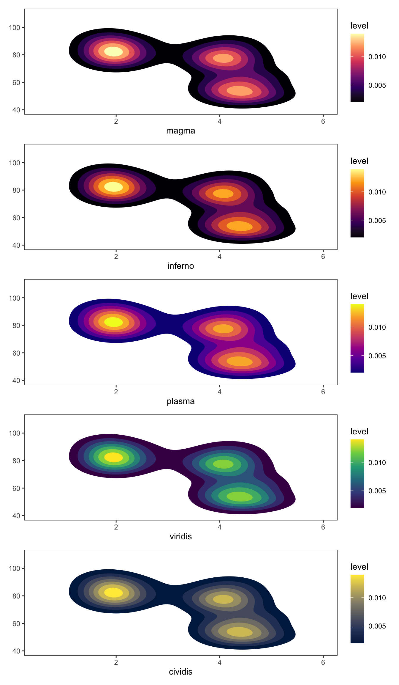

Let’s see what the PRISM tmax maps look like using Option A and D (default). Since the aesthetics type is fill and tmax is continuous, scale_fill_viridis_c() is the appropriate one here.

g_col_scale + scale_fill_viridis_c(option = "A")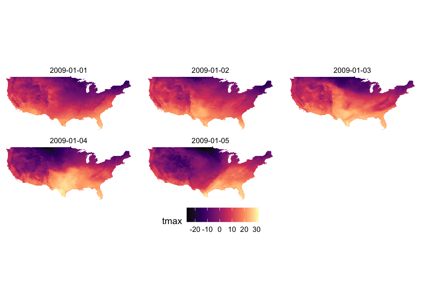

g_col_scale + scale_fill_viridis_c(option = "D")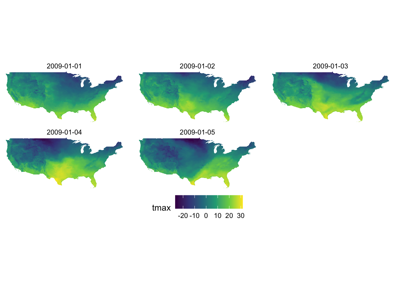

You can reverse the order of the color by adding direction = -1.

g_col_scale + scale_fill_viridis_c(option = "D", direction = -1)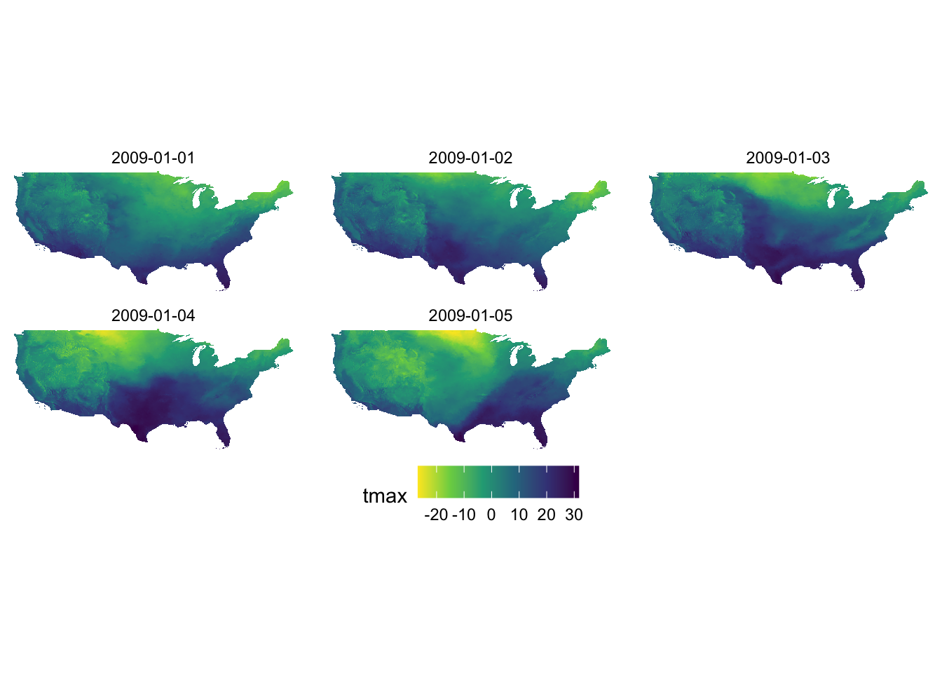

Let’s now work on aesthetics mapping based on a discrete variable. The code below groups af_used into five groups of ranges.

#--- convert af_used to a discrete variable ---#
gw_Stevens <- mutate(gw_Stevens, af_used_cat = cut_number(af_used, n = 5))

#--- take a look ---#
head(gw_Stevens)

Source: local data table [6 x 5]
Call:   head(copy(`_DT1`)[, `:=`(af_used_cat = cut_number(af_used, n = 5))], 
    n = 6L)

  well_id  year af_used             geometry af_used_cat   
    <dbl> <dbl>   <dbl>          <POINT [°]> <fct>         
1     234  2010    462.  (-101.4232 37.1165) (377,508]     
2     234  2011    486.  (-101.4232 37.1165) (377,508]     
3     290  2010    457. (-101.2301 37.29295) (377,508]     
4     290  2011    580. (-101.2301 37.29295) (508,1.19e+03]
5     317  2010    258  (-101.1111 37.04683) (157,264]     
6     317  2011    255  (-101.1111 37.04683) (157,264]     

# Use as.data.table()/as.data.frame()/as_tibble() to access results

Since we would like to control color aesthetics based on a discrete variable, we should be using scale_color_viridis_d().

ggplot(data = gw_Stevens) +
  geom_sf(aes(color = af_used_cat), size = 2) +
  scale_color_viridis_d(option = "C")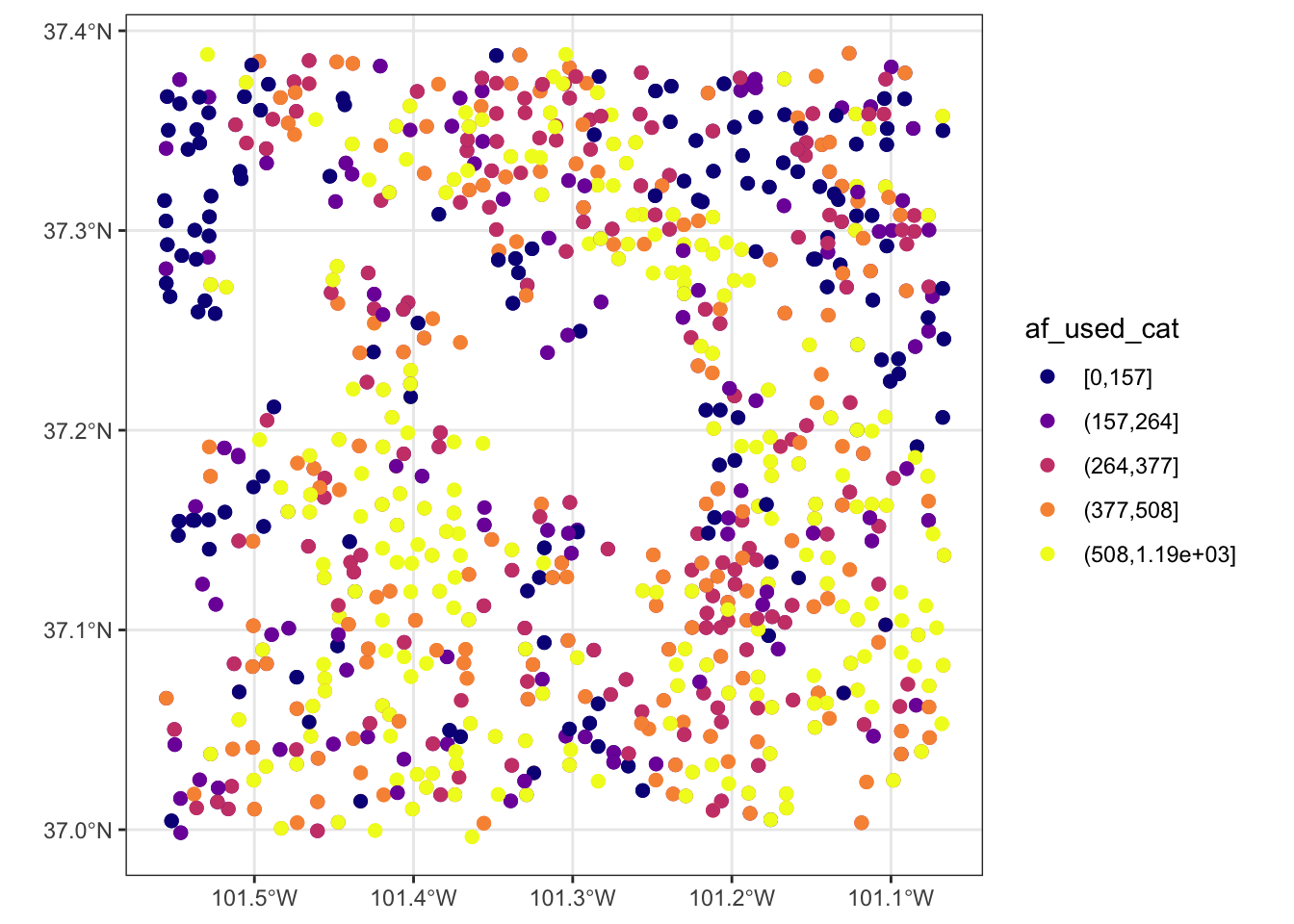

8.3.2 `RColorBrewer`: `scale__distiller()` and `scale__brewer()`

The RColorBrewer package provides a set of color scales that are useful. Here is the list of color scales you can use.

#--- load RColorBrewer ---#
library(RColorBrewer)

#--- disply all the color schemes from the package ---#
display.brewer.all()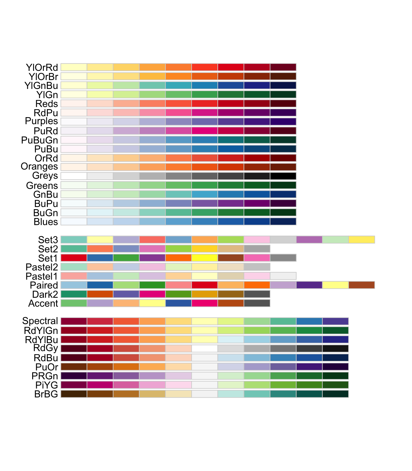

The first set of color palettes are sequential palettes and are suitable for a variable that has ordinal meaning: temperature, precipitation, etc. The second set of palettes are qualitative palettes and suitable for qualitative or categorical data. Finally, the third set of palettes are diverging palettes and can be suitable for variables that take both negative and positive values like changes in groundwater level.

Two types of scale functions can be used to use these palettes:

scale_*_distiller() for a continuous variable
scale_*_brewer() for a discrete variable

To use a specific color palette, you can simply add palette = "palette name" inside scale_fill_distiller(). The codes below applies “Spectral” as an example.

g_col_scale + theme_void() +
  scale_fill_distiller(palette = "Spectral")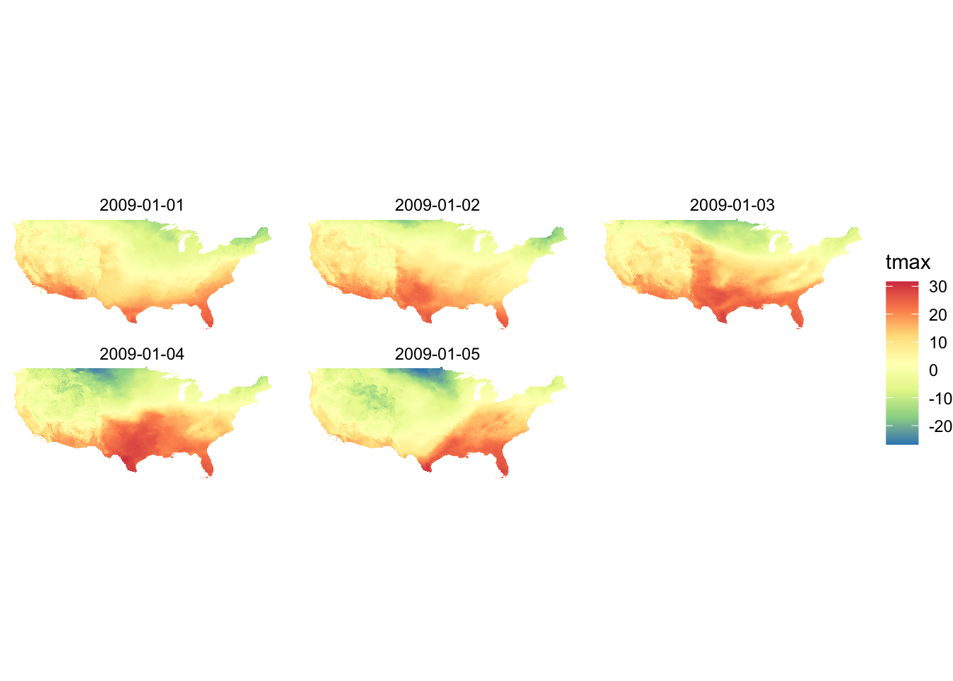

You can reverse the color order by adding trans = "reverse" option.

g_col_scale + theme_void() +
  scale_fill_distiller(palette = "Spectral", trans = "reverse")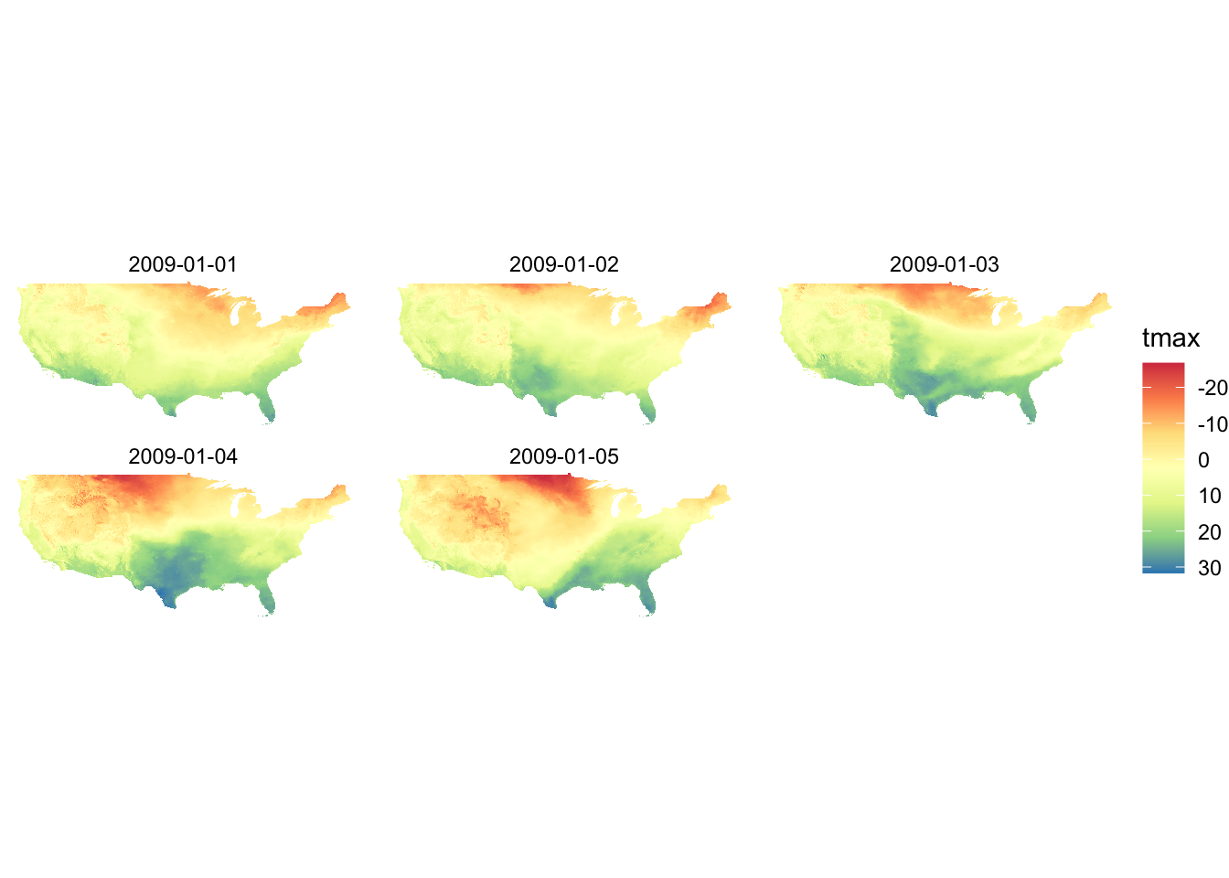

If you are specifying the color aesthetics based on a continuous variable, then you use scale_color_distiller().

ggplot(data = gw_Stevens) +
  geom_sf(aes(color = af_used), size = 2) +
  scale_color_distiller(palette = "Spectral")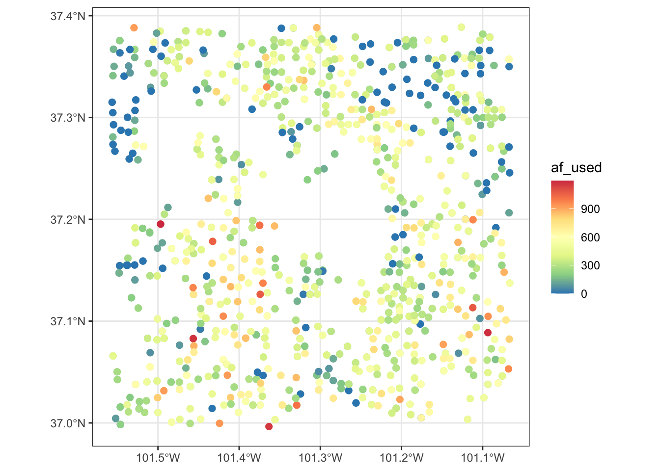

Now, suppose the variable of interest comes with categories of ranges of values. The code below groups af_used into five ranges using ggplo2::cut_number().

gw_Stevens <- mutate(gw_Stevens, af_used_cat = cut_number(af_used, n = 5))

Since af_used_cat is a discrete variable, you can use scale_color_brewer() instead.

ggplot(data = gw_Stevens) +
  geom_sf(aes(color = af_used_cat), size = 2) +
  scale_color_brewer(palette = "Spectral")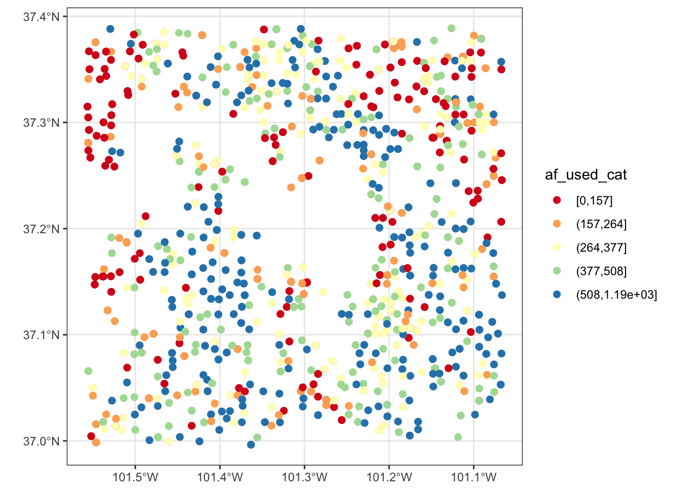

8.3.3 `colorspace` package

If you are not satisfied with the viridis color map or the ColorBrewer palette options, you might want to try the colorspace package.

Here is the palettes the colorspace package offers.

#--- plot the palettes ---#
hcl_palettes(plot = TRUE)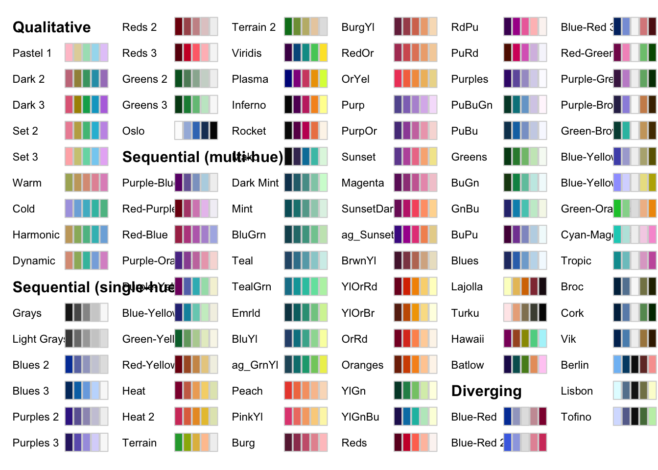

The packages offers its own scale_*() functions that follows the following naming convention:

scale_aesthetic_datatype_colorscale where

aesthetic: fill or color
datatype: continuous or discrete
colorscale: qualitative, sequential, diverging, divergingx

For example, to add a sequential color scale to the following map, we would use scale_fill_continuous_sequential() and then pick a palette from the set of sequential palettes shown above. The code below uses the Viridis palette with the reverse option:

ggplot() +
  geom_sf(data = gw_by_county, aes(fill = af_used)) +
  facet_wrap(. ~ year) +
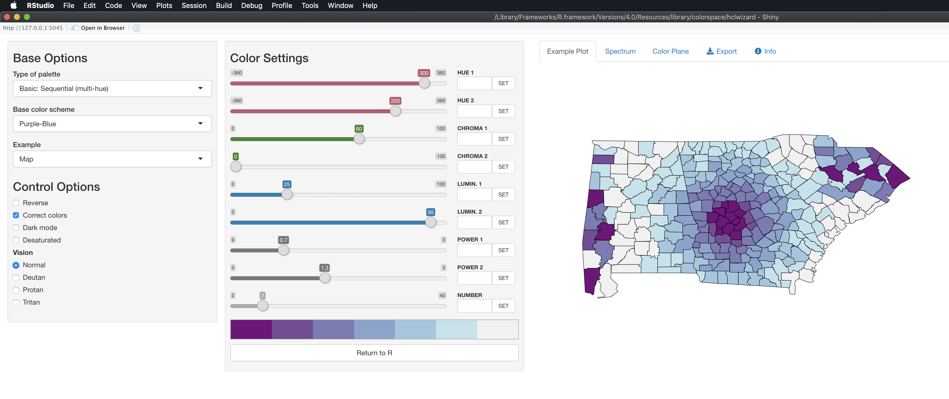
  scale_fill_continuous_sequential(palette = "Viridis", trans = "reverse")

If you still cannot find a palette that satisfies your need (or obsession at this point), then you can easily make your own. The package offers hclwizard(), which starts shiny-based web application to let you design your own color palette.

After running this,

hclwizard()

you should see a web application pop up that looks like this.

After you find a color scale you would like to use, you can go to the Exporttab, select the R tab, and then copy the code that appear in the highlighted area.

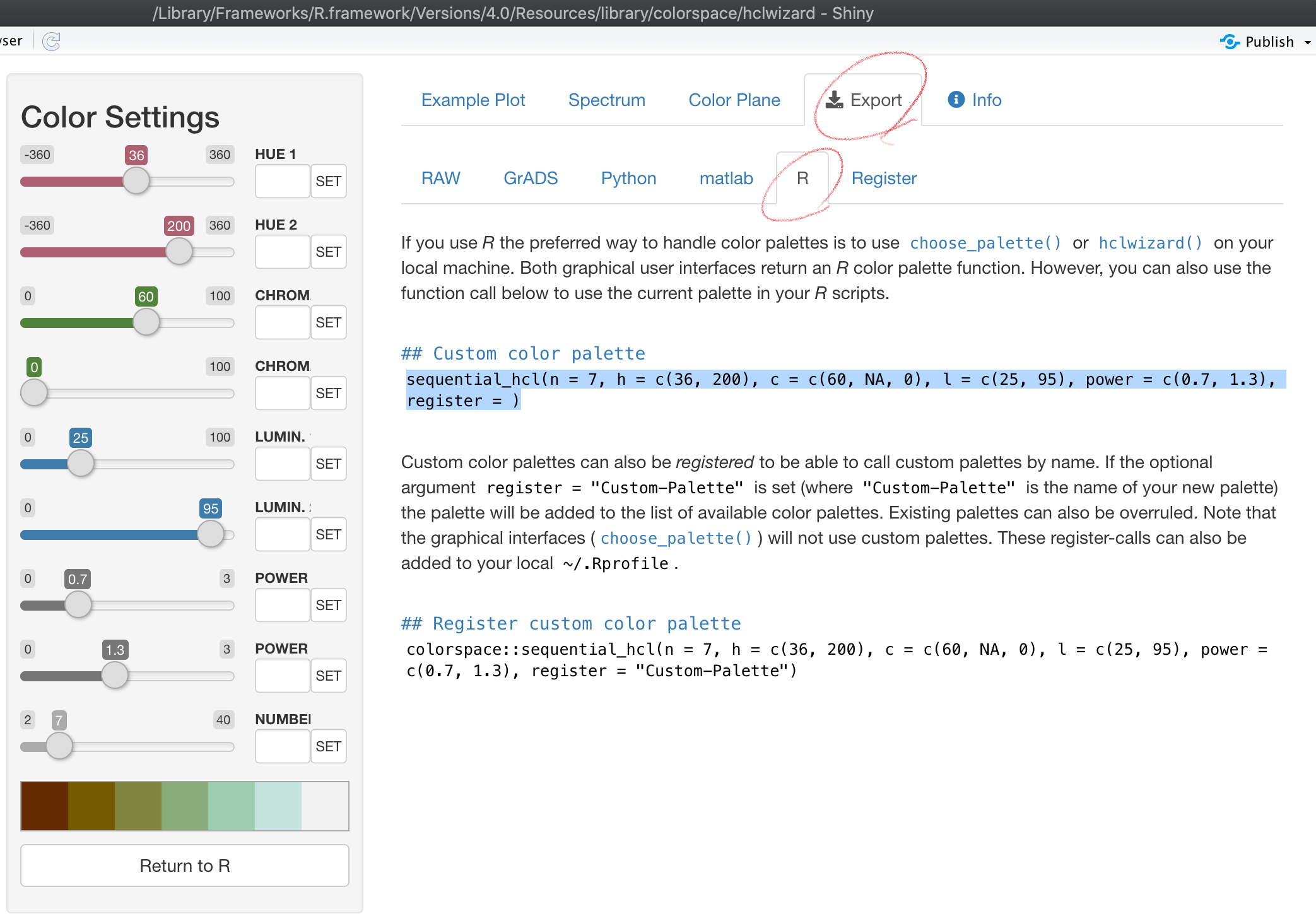
You could register the color palette by completing the register = option in the copied code if you think you will use it other times. Otherwise, you can delete the option.

col_palette <- sequential_hcl(n = 7, h = c(36, 200), c = c(60, NA, 0), l = c(25, 95), power = c(0.7, 1.3))

We then use the code as follows:

g_col_scale + theme_void() +
  scale_fill_gradientn(colors = col_palette)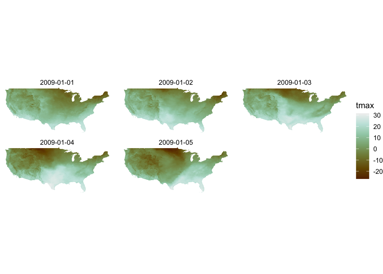

Note that you are now using scale_*_gradientn() with this approach.

For a discrete variable, you can use scale_*_manual():

col_discrete <- sequential_hcl(n = 5, h = c(240, 130), c = c(30, NA, 33), l = c(25, 95), power = c(1, NA), rev = TRUE)

ggplot() +
  geom_sf(data = gw_Stevens, aes(color = af_used_cat), size = 2) +
  scale_color_manual(values = col_discrete)

8.3 Color scale

8.3.1 Viridis color maps

8.3.2 RColorBrewer: scale_*_distiller() and scale_*_brewer()

8.3.3 colorspace package

8.3.2 `RColorBrewer`: `scale__distiller()` and `scale__brewer()`

8.3.3 `colorspace` package