9.4 Daymet with daymetr and FedData

For this section, we use the daymetr (Hufkens et al. 2018) and FedData packages (Bocinsky 2016).

library(daymetr)  
library(FedData)  

Daymet data consists of “tiles,” each of which consisting of raster cells of 1km by 1km. Here is the map of the tiles (Figure 9.3)

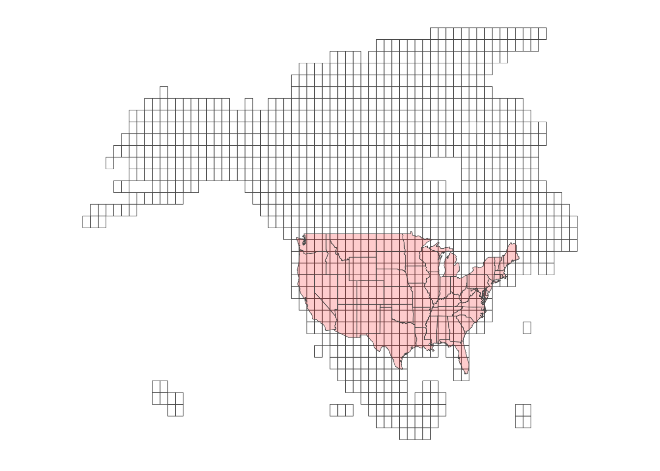
Figure 9.3: Daymet Tiles

Here is the list of weather variables:

• vapor pressure
• minimum and maximum temperature
• snow water equivalent
• solar radiation
• precipitation
  
• day length

So, Daymet provides information about more weather variables than PRISM, which helps to find some weather-dependent metrics, such as evapotranspiration.

The easiest way find Daymet values for your vector data depends on whether it is points or polygons data. For points data, daymetr::download_daymet() is the easiest because it will directly return weather values to the point of interest. Internally, it finds the cell in which the point is located, and then return the values of the cell for the specified length of period. daymetr::download_daymet() does all this for you. For polygons, we need to first download pertinent Daymet data for the region of interest first and then extract values for each of the polygons ourselves, which we learned in Chapter 5. Unfortunately, the netCDF data downloaded from daymetr::download_daymet_ncss() cannot be easily read by the raster package nor the stars package. On the contrary, FedData::get_daymet() download the the requested Daymet data and save it as a RasterBrick object, which can be easily turned into stars object using st_as_stars().

9.4.1 For points data

For points data, the easiest way to associate daily weather values to them is to use download_daymet(). download_daymet() can download daily weather data for a single point at a time by finding which cell of a tile the point is located within.

Here are key parameters for the function:

• lat: latitude
• lon: longitude
• start: start_year
• end: end_year
• internal: TRUE (dafault) or FALSE

For example, the code below downloads daily weather data for a point (lat = \(36\), longitude = \(-100\)) starting from 2000 to 2002 and assigns the downloaded data to temp_daymet.

#--- download daymet data ---#
temp_daymet <- download_daymet(
  lat = 36,
  lon = -100,
  start = 2000,
  end = 2002
) 

#--- structure ---#
str(temp_daymet)

List of 7
 $ site     : chr "Daymet"
 $ tile     : num 11380
 $ latitude : num 36
 $ longitude: num -100
 $ altitude : num 746
 $ tile     : num 11380
 $ data     :'data.frame':  1095 obs. of  9 variables:
  ..$ year         : int [1:1095] 2000 2000 2000 2000 2000 2000 2000 2000 2000 2000 ...
  ..$ yday         : int [1:1095] 1 2 3 4 5 6 7 8 9 10 ...
  ..$ dayl..s.     : num [1:1095] 34571 34606 34644 34685 34729 ...
  ..$ prcp..mm.day.: num [1:1095] 0 0 0 0 0 0 0 0 0 0 ...
  ..$ srad..W.m.2. : num [1:1095] 334 231 148 319 338 ...
  ..$ swe..kg.m.2. : num [1:1095] 18.2 15 13.6 13.6 13.6 ...
  ..$ tmax..deg.c. : num [1:1095] 20.9 13.88 4.49 9.18 13.37 ...
  ..$ tmin..deg.c. : num [1:1095] -2.73 1.69 -2.6 -10.16 -8.97 ...
  ..$ vp..Pa.      : num [1:1095] 500 690 504 282 310 ...
 - attr(*, "class")= chr "daymetr"

As you can see, temp_daymet has bunch of site information other than the download Daymet data.

#--- get the data part ---#
temp_daymet_data <- temp_daymet$data

#--- take a look ---#
head(temp_daymet_data)

  year yday dayl..s. prcp..mm.day. srad..W.m.2. swe..kg.m.2. tmax..deg.c.
1 2000    1 34571.11             0       334.34        18.23        20.90
2 2000    2 34606.19             0       231.20        15.00        13.88
3 2000    3 34644.13             0       148.29        13.57         4.49
4 2000    4 34684.93             0       319.13        13.57         9.18
5 2000    5 34728.55             0       337.67        13.57        13.37
6 2000    6 34774.96             0       275.72        13.11         9.98
  tmin..deg.c. vp..Pa.
1        -2.73  499.56
2         1.69  689.87
3        -2.60  504.40
4       -10.16  282.35
5        -8.97  310.05
6        -4.89  424.78

As you might have noticed, yday is not the date of each observation, but the day of the year. You can easily convert it into dates like this:

temp_daymet_data <- mutate(temp_daymet_data, date = as.Date(paste(year, yday, sep = "-"), "%Y-%j"))

One dates are obtained, you can use the lubridate package to extract day, month, and year using day(), month(), and year(), respectively.

library(lubridate)

temp_daymet_data <- mutate(temp_daymet_data,
  day = day(date),
  month = month(date),
  #--- this is already there though ---#
  year = year(date)
)

#--- take a look ---#
dplyr::select(temp_daymet_data, year, month, day) %>%  head

  year month day
1 2000     1   1
2 2000     1   2
3 2000     1   3
4 2000     1   4
5 2000     1   5
6 2000     1   6

This helps you find group statistics like monthly precipitation.

temp_daymet_data %>% 
  group_by(month) %>% 
  summarize(prcp = mean(prcp..mm.day.))

# A tibble: 12 × 2
   month  prcp
   <dbl> <dbl>
 1     1 0.762
 2     2 1.20 
 3     3 2.08 
 4     4 1.24 
 5     5 3.53 
 6     6 3.45 
 7     7 1.78 
 8     8 1.19 
 9     9 1.32 
10    10 4.78 
11    11 0.407
12    12 0.743

Downloading Daymet data for many points is just applying the same operations above to them using a loop. Let’s create random points within California and get their coordinates.

set.seed(389548)

random_points <- 
  tigris::counties(state = "CA") %>% 
  st_as_sf() %>% 
  #--- 10 points ---#
  st_sample(10) %>% 
  #--- get the coordinates ---#
  st_coordinates() %>% 
  #--- as tibble (data.frame) ---#
  as_tibble() %>% 
  #--- assign site id ---#
  mutate(site_id = 1:n())

To loop over the points, you can first write a function like this:

get_daymet <- function(i){

  temp_lat <- random_points[i, ] %>% pull(Y)
  temp_lon <- random_points[i, ] %>% pull(X)
  temp_site <- random_points[i, ] %>% pull(site_id)

  temp_daymet <- download_daymet(
    lat = temp_lat,
    lon = temp_lon,
    start = 2000,
    end = 2002
  ) %>% 
  #--- just get the data part ---#
  .$data %>% 
  #--- convert to tibble (not strictly necessary) ---#
  as_tibble() %>% 
  #--- assign site_id so you know which record is for which site_id ---#
  mutate(site_id = temp_site) %>% 
  #--- get date from day of the year ---#
  mutate(date = as.Date(paste(year, yday, sep = "-"), "%Y-%j"))

  return(temp_daymet)
}  

Here is what the function returns for the 1st row of random_points:

get_daymet(1)

# A tibble: 1,095 × 11
    year  yday dayl..s. prcp..mm.day. srad..W.m.2. swe..kg.m.2. tmax..deg.c.
   <int> <int>    <dbl>         <dbl>        <dbl>        <dbl>        <dbl>
 1  2000     1   34131.             0         246.            0         7.02
 2  2000     2   34168.             0         251.            0         4.67
 3  2000     3   34208.             0         247.            0         7.32
 4  2000     4   34251              0         267.            0        10   
 5  2000     5   34297              0         240.            0         4.87
 6  2000     6   34346.             0         274.            0         7.79
 7  2000     7   34398.             0         262.            0         7.29
 8  2000     8   34453.             0         291.            0        11.2 
 9  2000     9   34510.             0         268.            0        10.0 
10  2000    10   34570.             0         277.            0        11.8 
# … with 1,085 more rows, and 4 more variables: tmin..deg.c. <dbl>,
#   vp..Pa. <dbl>, site_id <int>, date <date>

You can now simply loop over the rows.

(
daymet_all_points <- lapply(1:nrow(random_points), get_daymet) %>% 
  #--- need to combine the list of data.frames into a single data.frame ---#
  bind_rows()
)

# A tibble: 10,950 × 11
    year  yday dayl..s. prcp..mm.day. srad..W.m.2. swe..kg.m.2. tmax..deg.c.
   <dbl> <dbl>    <dbl>         <dbl>        <dbl>        <dbl>        <dbl>
 1  2000     1   33523.             0         230.            0         12  
 2  2000     2   33523.             0         240             0         11.5
 3  2000     3   33523.             0         243.            0         13.5
 4  2000     4   33523.             1         230.            0         13  
 5  2000     5   33523.             0         243.            0         14  
 6  2000     6   33523.             0         243.            0         13  
 7  2000     7   33523.             0         246.            0         14  
 8  2000     8   33869.             0         230.            0         13  
 9  2000     9   33869.             0         227.            0         12.5
10  2000    10   33869.             0         214.            0         14  
# … with 10,940 more rows, and 4 more variables: tmin..deg.c. <dbl>,
#   vp..Pa. <dbl>, site_id <int>, date <date>

Or better yet, you can easily parallelize this process as follows (see Chapter A if you are not familiar with parallelization in R):

library(future.apply)    
library(parallel)

#--- parallelization planning ---#
plan(multiprocess, workers = detectCores() - 1)

#--- parallelized lapply ---#
daymet_all_points <- future_lapply(1:nrow(random_points), get_daymet) %>% 
  #--- need to combine the list of data.frames into a single data.frame ---#
  bind_rows()

9.4.2 For polygons data

Suppose you are interested in getting Daymet data for select counties in Michigan (Figure 9.4).

#--- entire MI ---#
MI_counties <- tigris::counties(state = "MI")

#--- select counties ---#
MI_counties_select <- filter(MI_counties, NAME %in% c("Luce", "Chippewa", "Mackinac"))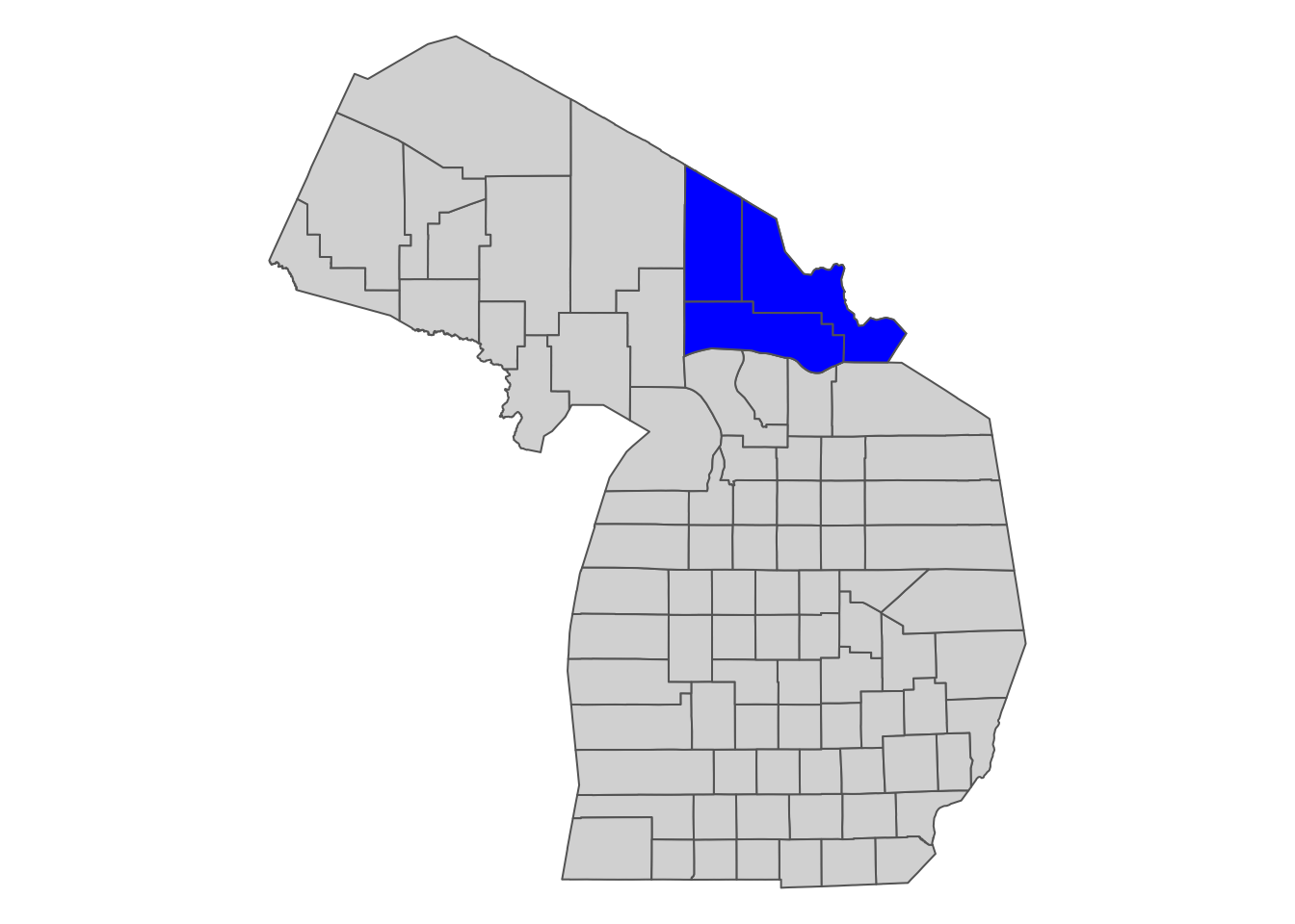

Figure 9.4: Select Michigan counties for which we download Daymet data

We can use FedData::get_daymet() to download Daymet data that covers the spatial extent of the polygons data. The downloaded dataset can be assigned to an R object as RasterBrick (you could alternatively write the downloaded data to a file). In order to let the function know the spatial extent for which it download Daymet data, we supply a SpatialPolygonsDataFrame object supported by the sp package. Since our main vector data handling package is sf we need to convert the sf object to a sp object.

The code below downloads prcp and tmax for the spatial extent of Michigan counties for 2000 and 2001:

(
MI_daymet_select <- FedData::get_daymet(
  #--- supply the vector data in sp ---#
  template = as(MI_counties_select, "Spatial"),
  #--- label ---#
  label = "MI_counties_select",
  #--- variables to download ---#
  elements = c("prcp","tmax"),
  #--- years ---#
  years = 2000:2001
)
)

$prcp
class      : RasterBrick 
dimensions : 96, 156, 14976, 730  (nrow, ncol, ncell, nlayers)
resolution : 1000, 1000  (x, y)
extent     : 1027250, 1183250, 455500, 551500  (xmin, xmax, ymin, ymax)
crs        : +proj=lcc +lon_0=-100 +lat_0=42.5 +x_0=0 +y_0=0 +lat_1=25 +lat_2=60 +ellps=WGS84 
source     : memory
names      : X2000.01.01, X2000.01.02, X2000.01.03, X2000.01.04, X2000.01.05, X2000.01.06, X2000.01.07, X2000.01.08, X2000.01.09, X2000.01.10, X2000.01.11, X2000.01.12, X2000.01.13, X2000.01.14, X2000.01.15, ... 
min values :           0,           0,           0,           0,           0,           0,           0,           0,           0,           0,           0,           0,           0,           0,           0, ... 
max values :           6,          26,          19,          17,           6,           9,           6,           1,           0,          13,          15,           6,           0,           4,           7, ... 


$tmax
class      : RasterBrick 
dimensions : 96, 156, 14976, 730  (nrow, ncol, ncell, nlayers)
resolution : 1000, 1000  (x, y)
extent     : 1027250, 1183250, 455500, 551500  (xmin, xmax, ymin, ymax)
crs        : +proj=lcc +lon_0=-100 +lat_0=42.5 +x_0=0 +y_0=0 +lat_1=25 +lat_2=60 +ellps=WGS84 
source     : memory
names      : X2000.01.01, X2000.01.02, X2000.01.03, X2000.01.04, X2000.01.05, X2000.01.06, X2000.01.07, X2000.01.08, X2000.01.09, X2000.01.10, X2000.01.11, X2000.01.12, X2000.01.13, X2000.01.14, X2000.01.15, ... 
min values :         0.5,        -4.5,        -8.0,        -8.5,        -7.0,        -2.5,        -6.5,        -1.5,         1.5,         2.0,        -1.5,        -8.5,       -14.0,        -9.5,        -3.0, ... 
max values :         3.0,         3.0,         0.5,        -2.5,        -2.5,         0.0,         0.5,         1.5,         4.0,         3.0,         3.5,         0.5,        -6.5,        -4.0,         0.0, ... 

As you can see, Daymet prcp and tmax data are stored separately as RasterBrick. Now that you have stars objects, you can extract values for your target polygons data using the methods described in Chapter 5.

If you use the stars package for raster data handling (see Chapter 7), you can convert them into stars object using st_as_stars().

#--- tmax as stars ---#
tmax_stars <- st_as_stars(MI_daymet_select$tmax)

#--- prcp as stars ---#
prcp_stars <- st_as_stars(MI_daymet_select$prcp)

Now, the third dimension (band) is not recognized as dates. We can use st_set_dimension() to change that (see Chapter 7.5). Before that, we first need to recover Date values from the “band” values as follows:

date_values <- tmax_stars %>% 
  #--- get band values ---#
  st_get_dimension_values(., "band") %>% 
  #--- remove X ---#
  gsub("X", "", .) %>% 
  #--- convert to date ---#
  ymd(.)

#--- take a look ---#
head(date_values)

[1] "2000-01-01" "2000-01-02" "2000-01-03" "2000-01-04" "2000-01-05"
[6] "2000-01-06"

#--- tmax ---#
st_set_dimensions(tmax_stars, 3, values = date_values, names = "date" )  

stars object with 3 dimensions and 1 attribute
attribute(s), summary of first 1e+05 cells:
             Min. 1st Qu. Median      Mean 3rd Qu. Max. NA's
X2000.01.01  -8.5      -4     -2 -1.884266       0    3  198
dimension(s):
     from  to  offset delta                       refsys point
x       1 156 1027250  1000 +proj=lcc +lon_0=-100 +la...    NA
y       1  96  551500 -1000 +proj=lcc +lon_0=-100 +la...    NA
date    1 730      NA    NA                         Date    NA
                        values x/y
x                         NULL [x]
y                         NULL [y]
date 2000-01-01,...,2001-12-31    

#--- prcp ---#
st_set_dimensions(prcp_stars, 3, values = date_values, names = "date" )  

stars object with 3 dimensions and 1 attribute
attribute(s), summary of first 1e+05 cells:
             Min. 1st Qu. Median     Mean 3rd Qu. Max. NA's
X2000.01.01     0       0      3 6.231649      12   26  198
dimension(s):
     from  to  offset delta                       refsys point
x       1 156 1027250  1000 +proj=lcc +lon_0=-100 +la...    NA
y       1  96  551500 -1000 +proj=lcc +lon_0=-100 +la...    NA
date    1 730      NA    NA                         Date    NA
                        values x/y
x                         NULL [x]
y                         NULL [y]
date 2000-01-01,...,2001-12-31    

Notice that the date dimension has NA for delta. This is because Daymet removes observations for December 31 in leap years to make the time dimension 365 consistently across years. This means that there is a one-day gap between “2000-12-30” and “2000-01-01” as you can see below:

date_values[364:367]

[1] "2000-12-29" "2000-12-30" "2001-01-01" "2001-01-02"

References

Bocinsky, R. Kyle. 2016. FedData: Functions to Automate Downloading Geospatial Data Available from Several Federated Data Sources. http://CRAN.R-project.org/package=FedData.

Hufkens, Koen, David Basler, Tom Milliman, Eli K. Melaas, and Andrew D. Richardson. 2018. “An Integrated Phenology Modelling Framework in r: Modelling Vegetation Phenology with phenor.” Methods in Ecology & Evolution 9: 1–10. http://onlinelibrary.wiley.com/doi/10.1111/2041-210X.12970/full.