6.1 Single raster layer
Let’s prepare for parallel processing for the rest of the section.
library(parallel)

#--- get the number of logical cores to use ---#
(
num_cores <- detectCores() - 1
)
[1] 156.1.1 Datasets
We will use the following datasets:
- raster: Iowa Cropland Data Layer (CDL) data in 2015
- polygons: Regular polygon grids over Iowa
Iowa CDL data in 2015
#--- Iowa CDL in 2015 ---#
(
IA_cdl_15 <- raster("Data/IA_cdl_2015.tif")
)
class : RasterLayer
dimensions : 11671, 17795, 207685445 (nrow, ncol, ncell)
resolution : 30, 30 (x, y)
extent : -52095, 481755, 1938165, 2288295 (xmin, xmax, ymin, ymax)
crs : +proj=aea +lat_0=23 +lon_0=-96 +lat_1=29.5 +lat_2=45.5 +x_0=0 +y_0=0 +ellps=GRS80 +units=m +no_defs
source : IA_cdl_2015.tif
names : IA_cdl_2015
values : 0, 229 (min, max)Values recorded in the raster data are integers representing land use type.
Regularly-sized grids over Iowa
#--- regular grids over Iowa ---#
(
IA_grids <- st_as_sf(map("state", "iowa", plot = FALSE, fill = TRUE)) %>%
  #--- create regularly-sized grids ---#
  st_make_grid(n = c(50, 50)) %>%
  #--- project to the CRS of the CDL data ---#
  st_transform(projection(IA_cdl_15)) %>%
  #--- convert to sf from sfc  ---#
  st_as_sf()
)
Simple feature collection with 2500 features and 0 fields
Geometry type: POLYGON
Dimension: XY
Bounding box: xmin: -51047.02 ymin: 1929141 xmax: 493167.9 ymax: 2294247
CRS: +proj=aea +lat_0=23 +lon_0=-96 +lat_1=29.5 +lat_2=45.5 +x_0=0 +y_0=0 +ellps=GRS80 +units=m +no_defs
First 10 features:
x
1 POLYGON ((-51047.02 1929303...
2 POLYGON ((-40156.64 1929241...
3 POLYGON ((-29266.18 1929194...
4 POLYGON ((-18375.66 1929162...
5 POLYGON ((-7485.114 1929144...
6 POLYGON ((3405.449 1929141,...
7 POLYGON ((14296 1929153, 25...
8 POLYGON ((25186.53 1929180,...
9 POLYGON ((36077.02 1929222,...
10 POLYGON ((46967.43 1929278,...Here is how they look (Figure 6.1):
tm_shape(IA_cdl_15) +
  tm_raster(title = "Land Use ") +
tm_shape(IA_grids) +
  tm_polygons(alpha = 0) +
tm_layout(legend.outside = TRUE)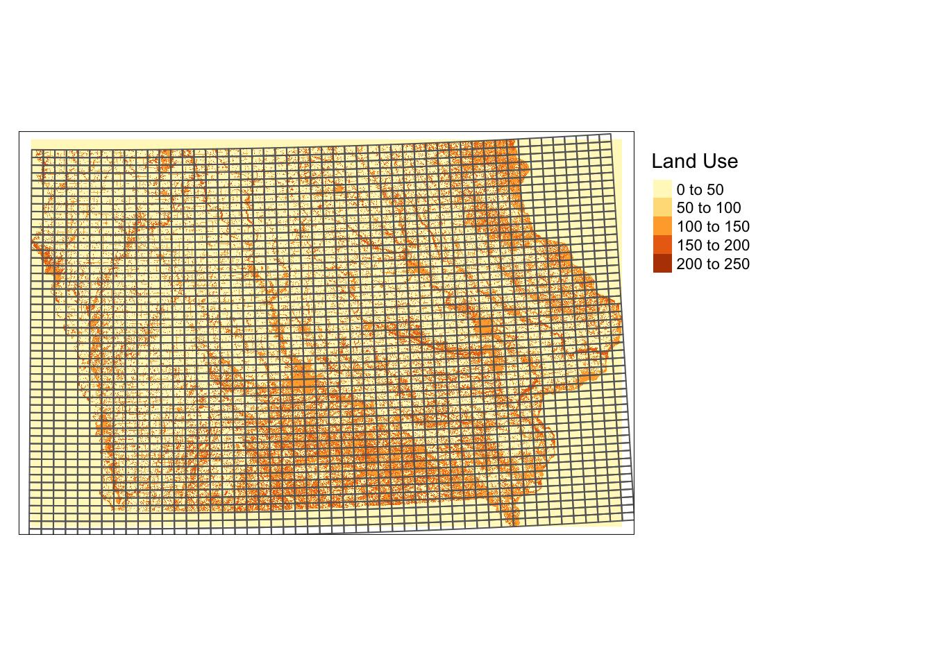
Figure 6.1: Regularly-sized grids and land use type in Iowa in 2105
6.1.2 Parallelization
Here is how long it takes to extract raster data values for the polygon grids using exact_extract().
tic()
temp <- exact_extract(IA_cdl_15, IA_grids)
toc()
elapsed
26.879 One way to parallelize this process is to let each core work on one polygon at a time. Let’s first define the function to extract values for one polygon and then run it for all the polygons parallelized.
#--- function to extract raster values for a single polygon ---#
get_values_i <- function(i){

  temp <- exact_extract(IA_cdl_15, IA_grids[i, ])

  return(temp)
}

#--- parallelized ---#
tic()
temp <- mclapply(1:nrow(IA_grids), get_values_i, mc.cores = num_cores)
toc()
elapsed
89.721 As you can see, this is a terrible way to parallelize the computation process. To see why, let’s look at the computation time of extracting from one polygon, two polygons, and up to five polygons.
library(microbenchmark)
mb <- microbenchmark(
  "p_1" = {
    temp <- exact_extract(IA_cdl_15, IA_grids[1, ])
  },
  "p_2" = {
    temp <- exact_extract(IA_cdl_15, IA_grids[1:2, ])
  },
  "p_3" = {
    temp <- exact_extract(IA_cdl_15, IA_grids[1:3, ])
  },
  "p_4" = {
    temp <- exact_extract(IA_cdl_15, IA_grids[1:4, ])
  },
  "p_5" = {
    temp <- exact_extract(IA_cdl_15, IA_grids[1:5, ])
  },
  times = 100
)
mb %>% data.table() %>%
.[, expr := gsub("p_", "", expr)] %>%
ggplot(.) +
geom_boxplot(aes(y = time/1e9, x = expr)) +
ylim(0, NA) +
ylab("seconds") +
xlab("number of polygons to process")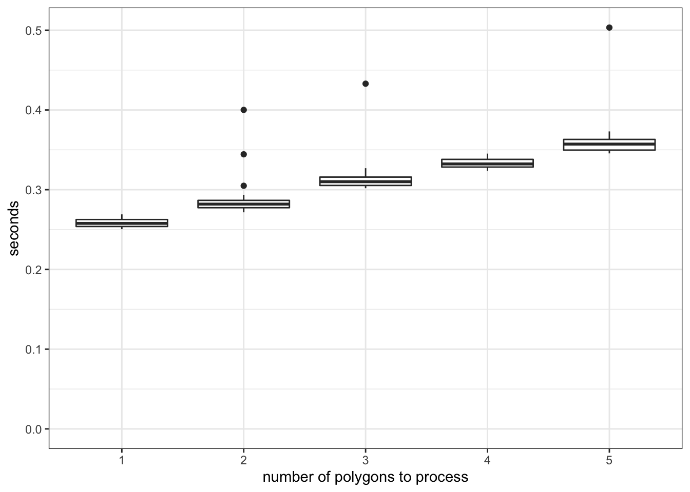
Figure 6.2: Comparison of the computation time of raster data extractions
As you can see in Figure 6.2, there is a significant overhead (about 0.23 seconds) irrespective of the number of the polygons to extract data for. Once the process is initiated and ready to start extracting values for polygons, it does not spend much time processing for additional units of polygon. So, this is a typical example of how you should NOT parallelize. Since each core processes about \(136\) polygons, a very simple math suggests that you would spend at least 31.28 (0.23 \(\times\) 136) seconds just for preparing extraction jobs.
We can minimize this overhead as much as possible by having each core use exact_extract() only once in which multiple polygons are processed in the single call. Specifically, we will split the collection of the polygons into 15 groups and have each core extract for one group.
#--- number of polygons in a group ---#
num_in_group <- floor(nrow(IA_grids)/num_cores)

#--- assign group id to polygons ---#
IA_grids <- IA_grids %>%
  mutate(
    #--- create grid id ---#
    grid_id = 1:nrow(.),
    #--- assign group id  ---#
    group_id = grid_id %/% num_in_group + 1
  )

tic()
#--- parallelized processing by group ---#
temp <- mclapply(
  1:num_cores,
  function(i) exact_extract(IA_cdl_15, filter(IA_grids, group_id == i)),
  mc.cores = num_cores
)
toc()
elapsed
11.901 Great, this is much better.76
Now, we can further reduce the processing time by reducing the size of the object that is returned from each core to be collated into one. In the code above, each core returns a list of data.frames where each grid of the same group has multiple values from the intersecting raster cells.
#--- take a look at the the values extracted for the 1st polygon of the 1st group---#
head(temp[[1]][[1]])
[1] "Error in (function (cond) : \n error in evaluating the argument 'y' in selecting a method for function 'exact_extract': Problem while computing `..1 = group_id == i`.\nCaused by error:\n! object 'group_id' not found\n"#--- the size of the list of data returned by the first core ---#
object.size(temp[[1]]) %>% format(units = "GB")[1] "0 Gb"In total, about 3GB of data has to be collated into one list from 15 cores. It turns out, this process is costly. To see this, take a look at the following example where the same exact_extrct() processes are run, yet nothing is returned by each core.
#--- define the function to extract values by block of polygons ---#
extract_by_group <- function(i){
  temp <- exact_extract(IA_cdl_15, filter(IA_grids, group_id == i))

  #--- returns nothing! ---#
  return(NULL)
}

#--- parallelized processing by group ---#
tic()
temp <- mclapply(
  1:num_cores,
  function(i) extract_by_group(i),
  mc.cores = num_cores
)
toc()
elapsed
6.689 Approximately 5.212 seconds were used just to collect the 3GB worth of data from the cores into one.
In most cases, we do not have to carry around all the individual cell values of landuse types for our subsequent analysis. For example, in Demonstration 3 (Chapter 1.3) we just need a summary (count) of each unique landuse type by polygon. So, let’s get the summary before we have the computer collect the objects returned from each core as follows:
extract_by_group_reduced <- function(i){

  temp_return <- exact_extract(
    IA_cdl_15,
    filter(IA_grids, group_id == i)
    ) %>%
    #--- combine the list of data.frames into one with polygon id ---#
    rbindlist(idcol = "id_within_group") %>%
    #--- find the count of land use type values by polygon ---#
    .[, .(num_value = .N), by = .(value, id_within_group)]

  return(temp_return)
}

tic()
#--- parallelized processing by group ---#
temp <- mclapply(
  1:num_cores,
  function(i) extract_by_group_reduced(i),
  mc.cores = num_cores
)
toc()
elapsed
8.514 It is of course slower than the one that returns nothing, but it is much faster than the one that does not reduce the size before the outcome collation.
As you can see, the computation time of the fastest approach is now much less, but you still only gained 81.21. How much time did I spend writing the code to do the parallelized group processing? Three minutes. Obviously, what matters to you is the total time (coding time plus processing time) you spend to get the desired outcome. Indeed, the time you could save by a clever coding at the most is 89.72 seconds. Writing any kind of code in an attempt to make your code faster takes more time than that. So, don’t even try to make your code faster if the processing time is quite short in the first place. Before you start parallelizing things, go through what you need to go through in terms of coding in your head, and judge if it’s worth it or not.
Imagine processing CDL data for all the states from 2009 to 2020. Then, the whole process will take roughly 15.25 (\(51 \times 12 \times 89.721/60/60\)) hours. Again, a super rough calculation tells us that the whole process would be done in 1.45 hours if parallelized in the same way as the best approach we saw above. While 15.25 is still not too terrible (you execute the program before you go to bed, and its results will be available in the afternoon the next day.), it is worth parallelizing this process even taking into account for the time you need to spend to code the parallelization process.
6.1.3 Summary
- Do not let each core runs small tasks over and over again (extracting raster values for one polygon at a time), or you will suffer from significant overhead.
- Blocking is one way to avoid the problem above.
- Reduce the size of the outcome of each core as much as possible to spend less time to simply collating them into one.
- Do not forget about the time you would spend on coding parallelized processes.
To get the total time, I should include the codes to generate group id. But, they are so quick that I did not time them.↩︎