3.2 Spatial Subsetting (or Flagging)
Spatial subsetting refers to operations that narrow down the geographic scope of a spatial object (source data) based on another spatial object (target data). We illustrate spatial subsetting using Kansas county borders, the boundary of the High-Plains Aquifer (HPA), and agricultural irrigation wells in Kansas.
First, let’s import all the files we will use in this section.
#--- Kansas county borders ---#
KS_counties <- readRDS("Data/KS_county_borders.rds")

#--- HPA boundary ---#
hpa <- st_read(dsn = "Data", layer = "hp_bound2010") %>%
  .[1, ] %>%
  st_transform(st_crs(KS_counties))

#--- all the irrigation wells in KS ---#
KS_wells <- readRDS("Data/Kansas_wells.rds") %>%
  st_transform(st_crs(KS_counties))

#--- US railroad ---#
rail_roads <- st_read(dsn = "Data", layer = "tl_2015_us_rails") %>%
  st_transform(st_crs(KS_counties))
3.2.1 polygons (source) vs polygons (target)
The following map (Figure 3.4) shows the Kansas portion of the HPA and Kansas counties.58
#--- add US counties layer ---#
tm_shape(KS_counties) +
  tm_polygons() +
#--- add High-Plains Aquifer layer ---#
tm_shape(hpa) +
  tm_fill(col = "blue", alpha = 0.3)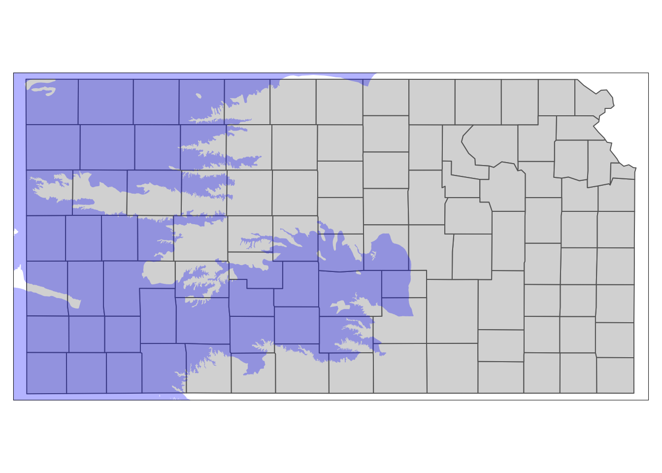
Figure 3.4: Kansas portion of High-Plains Aquifer and Kansas counties
The goal here is to select only the counties that intersect with the HPA boundary. When subsetting a data.frame by specifying the row numbers you would like to select, you can do
#--- this does not run ---#
data.frame[vector of row numbers, ]
Spatial subsetting of sf objects works in a similar syntax:
#--- this does not run ---#
sf_1[sf_2, ]
where you are subsetting sf_1 based on sf_2. Instead of row numbers, you provide another sf object in place. The following code spatially subsets Kansas counties based on the HPA boundary.
counties_in_hpa <- KS_counties[hpa, ]See the results below in Figure 3.5.
#--- add US counties layer ---#
tm_shape(counties_in_hpa) +
  tm_polygons() +
#--- add High-Plains Aquifer layer ---#
tm_shape(hpa) +
  tm_fill(col = "blue", alpha = 0.3)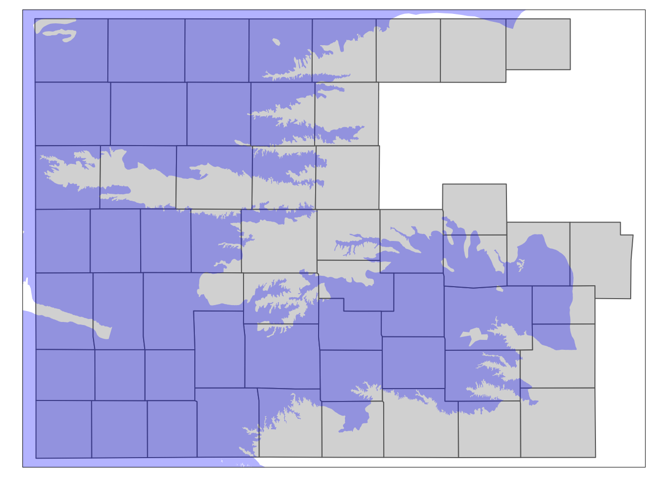
Figure 3.5: The results of spatially subsetting Kansas counties based on HPA boundary
You can see that only the counties that intersect with the HPA boundary remained. This is because when you use the above syntax of sf_1[sf_2, ], the default underlying topological relations is st_intersects(). So, if an object in sf_1 intersects with any of the objects in sf_2 even slightly, then it will remain after subsetting.
You can specify the spatial operation to be used as an option as in
#--- this does not run ---#
sf_1[sf_2, op = topological_relation_type]
For example, if you only want counties that are completely within the HPA boundary, you can do the following (the map of the results in Figure 3.6):
counties_within_hpa <- KS_counties[hpa, , op = st_within]#--- add US counties layer ---#
tm_shape(counties_within_hpa) +
tm_polygons() +
#--- add High-Plains Aquifer layer ---#
tm_shape(hpa) +
tm_fill(col = "blue", alpha = 0.3)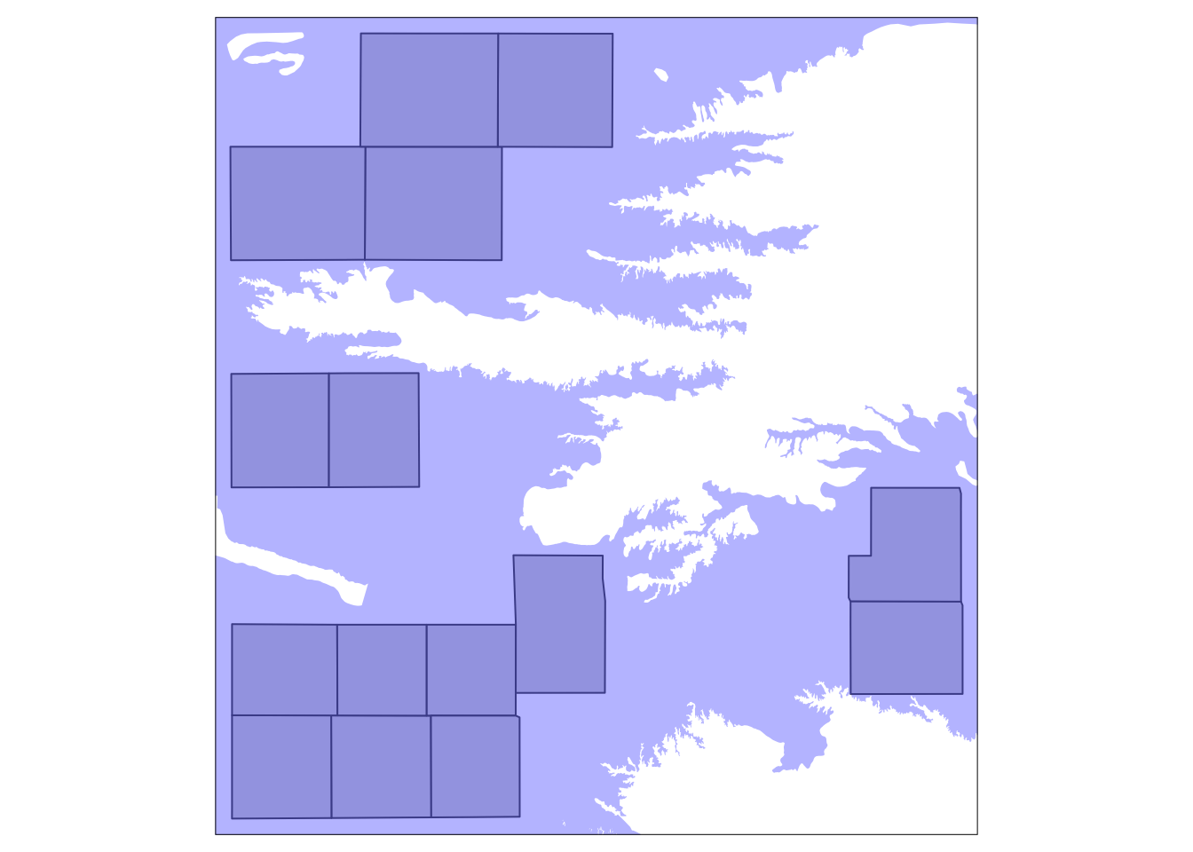
Figure 3.6: Kansas counties that are completely within the HPA boundary
Sometimes, you just want to flag whether two spatial objects intersect or not, instead of dropping non-overlapping observations. In that case, you can use st_intersects().
#--- check the intersections of HPA and counties  ---#
intersects_hpa <- st_intersects(KS_counties, hpa, sparse = FALSE)

#--- take a look ---#
head(intersects_hpa)
[,1]
[1,] FALSE
[2,] TRUE
[3,] FALSE
[4,] TRUE
[5,] TRUE
[6,] TRUE#--- assign the index as a variable ---#
KS_counties <- mutate(KS_counties, intersects_hpa = intersects_hpa)
#--- take a look ---#
dplyr::select(KS_counties, COUNTYFP, intersects_hpa)Simple feature collection with 105 features and 2 fields
Geometry type: MULTIPOLYGON
Dimension: XY
Bounding box: xmin: -102.0517 ymin: 36.99308 xmax: -94.59193 ymax: 40.00308
Geodetic CRS: NAD83
First 10 features:
COUNTYFP intersects_hpa geometry
1 133 FALSE MULTIPOLYGON (((-95.5255 37...
2 075 TRUE MULTIPOLYGON (((-102.0446 3...
3 123 FALSE MULTIPOLYGON (((-98.48738 3...
4 189 TRUE MULTIPOLYGON (((-101.5566 3...
5 155 TRUE MULTIPOLYGON (((-98.47279 3...
6 129 TRUE MULTIPOLYGON (((-102.0419 3...
7 073 FALSE MULTIPOLYGON (((-96.52278 3...
8 023 TRUE MULTIPOLYGON (((-102.0517 4...
9 089 TRUE MULTIPOLYGON (((-98.50445 4...
10 059 FALSE MULTIPOLYGON (((-95.50827 3...3.2.2 points (source) vs polygons (target)
The following map (Figure 3.7) shows the Kansas portion of the HPA and all the irrigation wells in Kansas.
tm_shape(KS_wells) +
  tm_symbols(size = 0.1) +
tm_shape(hpa) +
tm_polygons(col = "blue", alpha = 0.1) 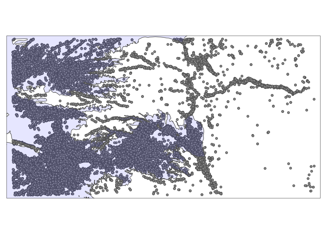
Figure 3.7: A map of Kansas irrigation wells and HPA
We can select only wells that reside within the HPA boundary using the same syntax as the above example.
KS_wells_in_hpa <- KS_wells[hpa, ]As you can see in Figure 3.8 below, only the wells that are inside (or intersect with) the HPA remained because the default topological relation is st_intersects().
tm_shape(KS_wells_in_hpa) +
  tm_symbols(size = 0.1) +
tm_shape(hpa) +
tm_polygons(col = "blue", alpha = 0.1) 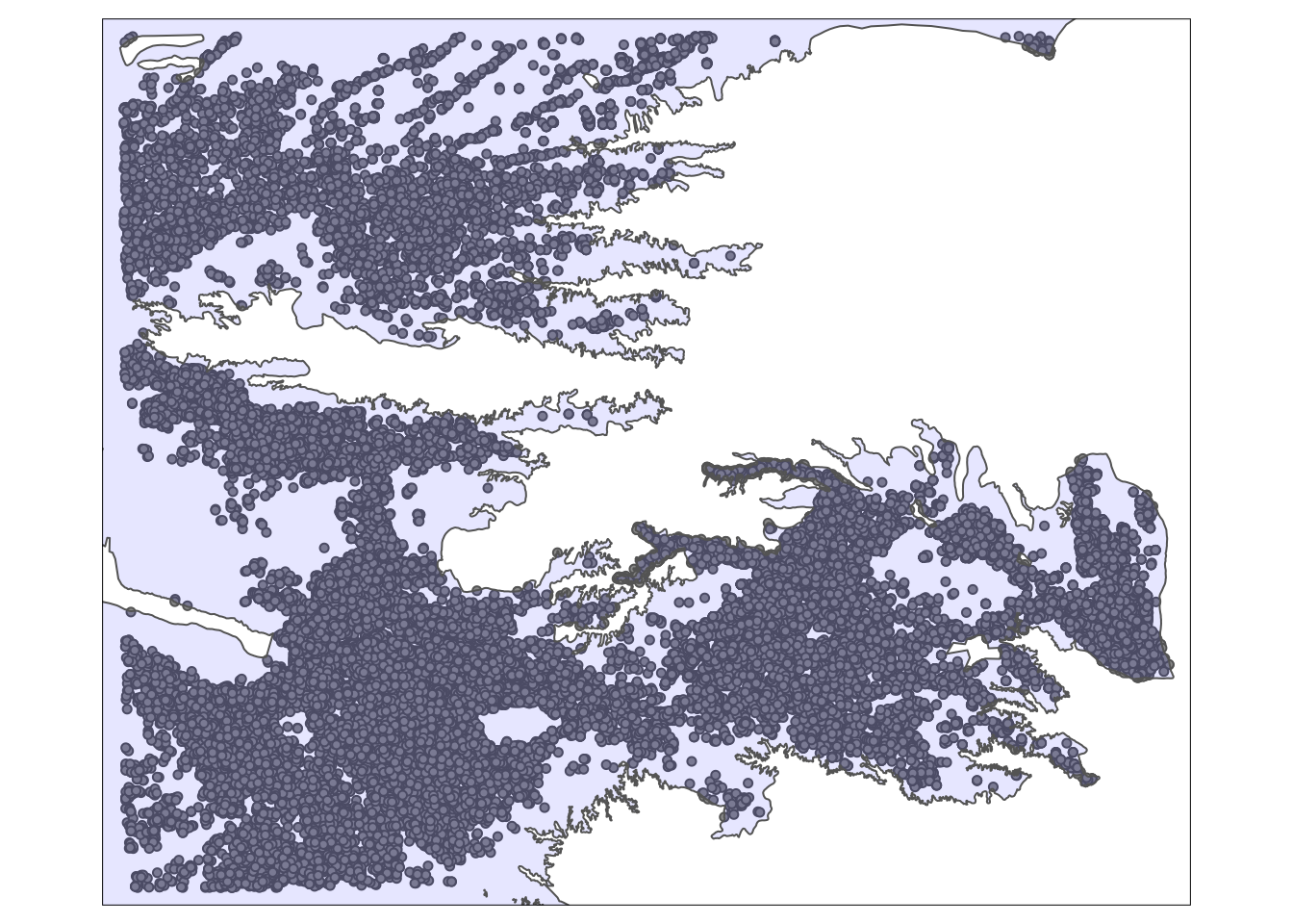
Figure 3.8: A map of Kansas irrigation wells and HPA
If you just want to flag wells that intersects with HPA instead of dropping the non-intersecting wells, use st_intersects():
(
KS_wells <- mutate(KS_wells, in_hpa = st_intersects(KS_wells, hpa, sparse = FALSE))
)
Simple feature collection with 37647 features and 3 fields
Geometry type: POINT
Dimension: XY
Bounding box: xmin: -102.0495 ymin: 36.99552 xmax: -94.62089 ymax: 40.00199
Geodetic CRS: NAD83
First 10 features:
site af_used geometry in_hpa
1 1 232.099948 POINT (-100.4423 37.52046) TRUE
2 3 13.183940 POINT (-100.7118 39.91526) TRUE
3 5 99.187052 POINT (-99.15168 38.48849) TRUE
4 7 0.000000 POINT (-101.8995 38.78077) TRUE
5 8 145.520499 POINT (-100.7122 38.0731) TRUE
6 9 3.614535 POINT (-97.70265 39.04055) FALSE
7 11 188.423543 POINT (-101.7114 39.55035) TRUE
8 12 77.335960 POINT (-95.97031 39.16121) FALSE
9 15 0.000000 POINT (-98.30759 38.26787) TRUE
10 17 167.819034 POINT (-100.2785 37.71539) TRUE3.2.3 lines (source) vs polygons (target)
The following map (Figure 3.9) shows the Kansas counties and U.S. railroads.
tm_shape(rail_roads) +
  tm_lines(col = "blue") +
tm_shape(KS_counties) +
  tm_polygons(alpha = 0)  +
tm_layout(frame = FALSE) 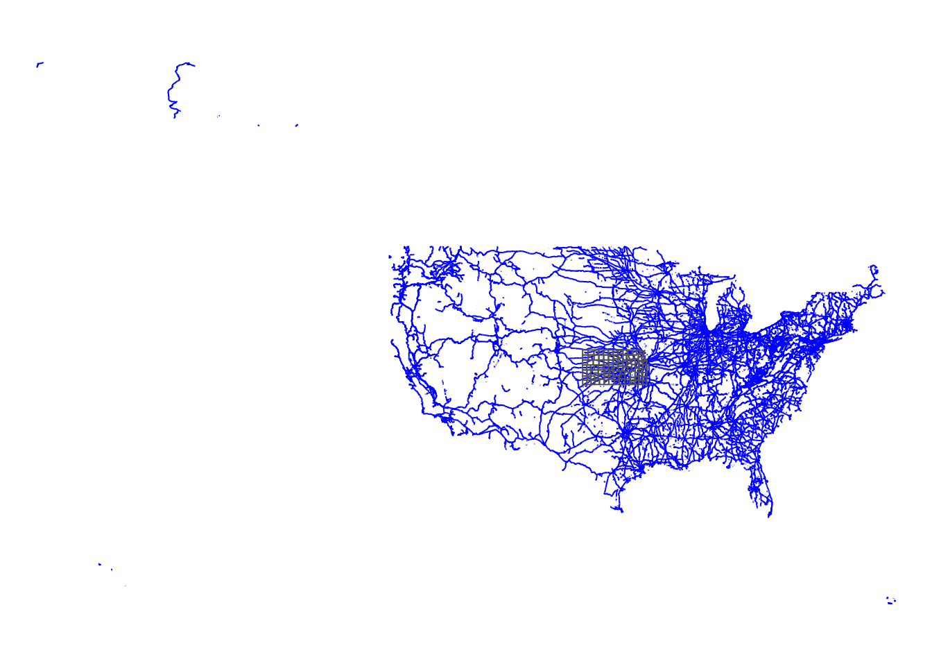
Figure 3.9: U.S. railroads and Kansas county boundaries
We can select only railroads that intersect with Kansas.
railroads_KS <- rail_roads[KS_counties, ]As you can see in Figure 3.10 below, only the railroads that intersect with Kansas were selected. Note the lines that go beyond the Kansas boundary are also selected. Remember, the default is st_intersect(). If you would like the lines beyond the state boundary to be cut out but the intersecting parts of those lines to remain, use st_intersection(), which is explained in Chapter 3.4.1.
tm_shape(railroads_KS) +
  tm_lines(col = "blue") +
tm_shape(KS_counties) +
  tm_polygons(alpha = 0)  +
tm_layout(frame = FALSE) 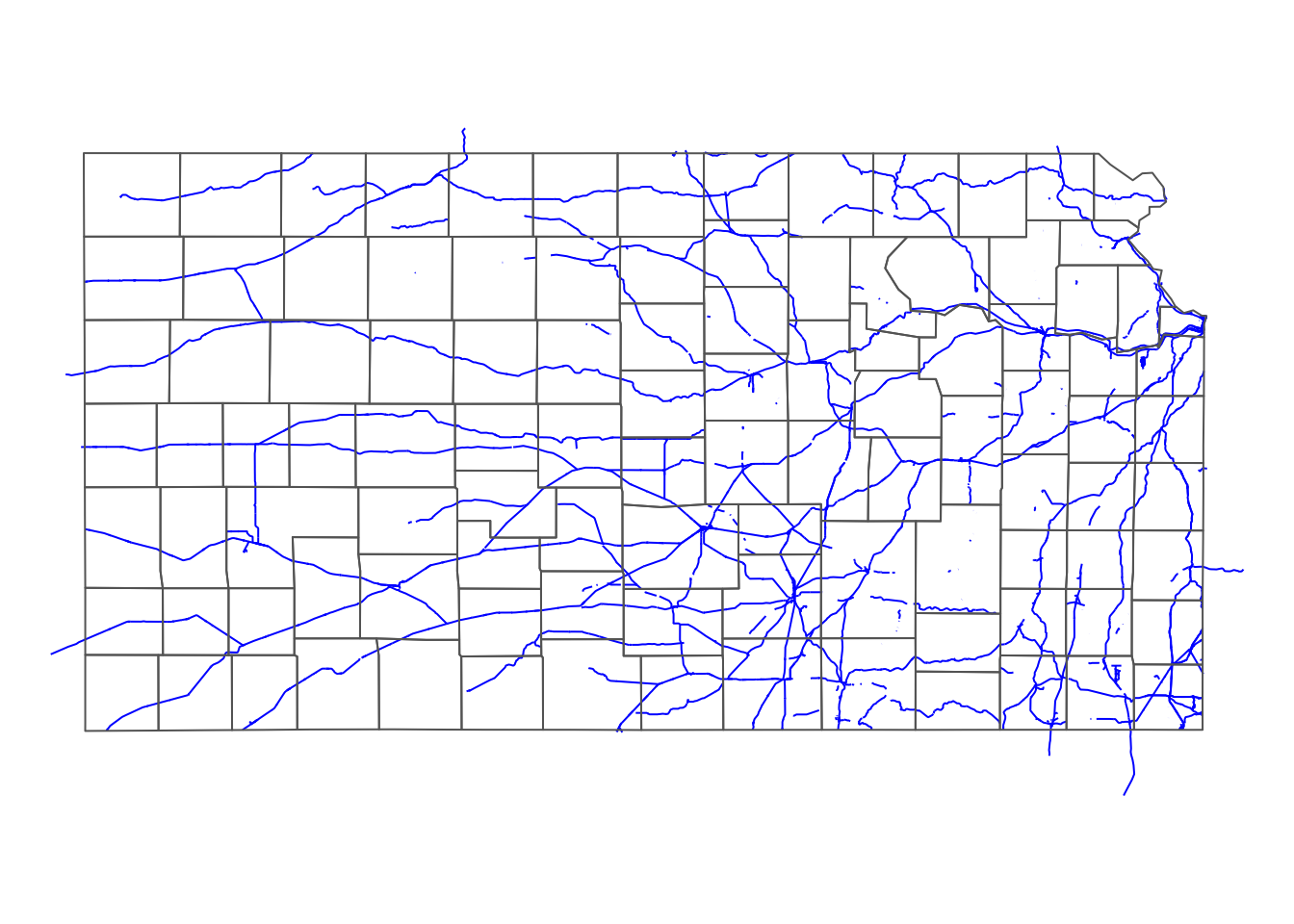
Figure 3.10: Railroads that intersect Kansas county boundaries
Unlike the previous two cases, multiple objects (lines) are checked against multiple objects (polygons) for intersection59. Therefore, we cannot use the strategy we took above of returning a vector of TRUE or FALSE using the sparse = TRUE option. Here, we count the number of intersecting counties and then assign TRUE if the number is greater than 0.
#--- check the number of intersecting KS counties ---#
int_mat <- st_intersects(rail_roads, KS_counties) %>%
  lapply(length) %>%
  unlist()

#--- railroads ---#
rail_roads <- mutate(rail_roads, intersect_ks  = int_mat > 0)

#--- take a look ---#
dplyr::select(rail_roads, LINEARID, intersect_ks)
Simple feature collection with 180958 features and 2 fields
Geometry type: MULTILINESTRING
Dimension: XY
Bounding box: xmin: -165.4011 ymin: 17.95174 xmax: -65.74931 ymax: 65.00006
Geodetic CRS: NAD83
First 10 features:
LINEARID intersect_ks geometry
1 11020239500 FALSE MULTILINESTRING ((-79.47058...
2 11020239501 FALSE MULTILINESTRING ((-79.46687...
3 11020239502 FALSE MULTILINESTRING ((-79.66819...
4 11020239503 FALSE MULTILINESTRING ((-79.46687...
5 11020239504 FALSE MULTILINESTRING ((-79.74031...
6 11020239575 FALSE MULTILINESTRING ((-79.43695...
7 11020239576 FALSE MULTILINESTRING ((-79.47852...
8 11020239577 FALSE MULTILINESTRING ((-79.43695...
9 11020239589 FALSE MULTILINESTRING ((-79.38736...
10 11020239591 FALSE MULTILINESTRING ((-79.53848...3.2.4 polygons (source) vs points (target)
The following map (Figure 3.11) shows the Kansas counties and irrigation wells in Kansas that overlie HPA.
tm_shape(KS_counties) +
  tm_polygons(alpha = 0) +
tm_shape(KS_wells_in_hpa) +
  tm_symbols(size = 0.1) +
  tm_layout(frame = FALSE)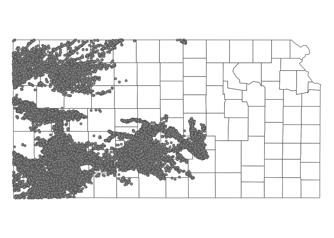
Figure 3.11: Kansas county boundaries and wells that overlie the HPA
We can select only counties that intersect with at least one well.
KS_counties_intersected <- KS_counties[KS_wells_in_hpa, ] As you can see in Figure 3.12 below, only the counties that intersect with at least one well remained.
tm_shape(KS_counties) +
  tm_polygons(col = NA) +
tm_shape(KS_counties_intersected) +
  tm_polygons(col ="blue", alpha = 0.6) +
  tm_layout(frame = FALSE)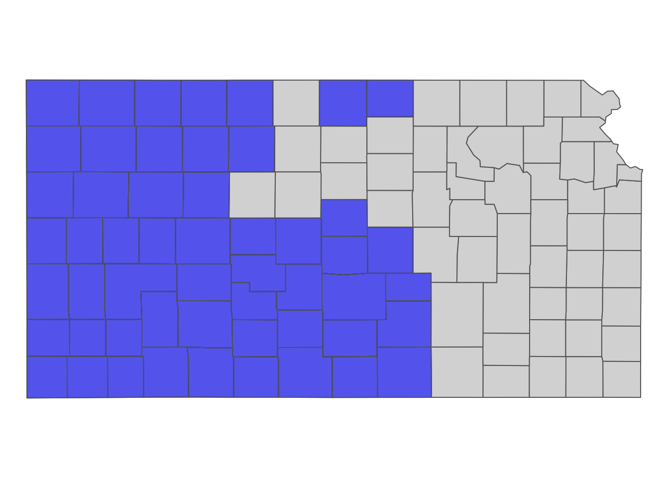
Figure 3.12: Counties that have at least one well
To flag counties that have at least one well, use st_intersects() as follows:
int_mat <- st_intersects(KS_counties, KS_wells_in_hpa) %>%
  lapply(length) %>%
  unlist()

#--- railroads ---#
KS_counties <- mutate(KS_counties, intersect_wells  = int_mat > 0)

#--- take a look ---#
dplyr::select(KS_counties, NAME, COUNTYFP, intersect_wells)
Simple feature collection with 105 features and 3 fields
Geometry type: MULTIPOLYGON
Dimension: XY
Bounding box: xmin: -102.0517 ymin: 36.99308 xmax: -94.59193 ymax: 40.00308
Geodetic CRS: NAD83
First 10 features:
NAME COUNTYFP intersect_wells geometry
1 Neosho 133 FALSE MULTIPOLYGON (((-95.5255 37...
2 Hamilton 075 TRUE MULTIPOLYGON (((-102.0446 3...
3 Mitchell 123 FALSE MULTIPOLYGON (((-98.48738 3...
4 Stevens 189 TRUE MULTIPOLYGON (((-101.5566 3...
5 Reno 155 TRUE MULTIPOLYGON (((-98.47279 3...
6 Morton 129 TRUE MULTIPOLYGON (((-102.0419 3...
7 Greenwood 073 FALSE MULTIPOLYGON (((-96.52278 3...
8 Cheyenne 023 TRUE MULTIPOLYGON (((-102.0517 4...
9 Jewell 089 TRUE MULTIPOLYGON (((-98.50445 4...
10 Franklin 059 FALSE MULTIPOLYGON (((-95.50827 3...3.2.5 Subsetting to a geographic extent (bounding box)
We can use st_crop() to crop spatial objects to a spatial bounding box (extent) of a spatial object. The bounding box of an sf is a rectangle represented by the minimum and maximum of x and y that encompass/contain all the spatial objects in the sf. You can use st_bbox() to find the bounding box of an sf object. Let’s get the bounding box of KS_wells_in_hpa (irrigation wells in Kansas that overlie HPA).
#--- get the bounding box of KS_wells ---#
(
bbox_KS_wells_in_hpa <- st_bbox(KS_wells_in_hpa)
)
xmin ymin xmax ymax
-102.04953 36.99552 -97.33193 40.00199 #--- check the class ---#
class(bbox_KS_wells_in_hpa)[1] "bbox"Visualizing the bounding box (Figure 3.13):
tm_shape(KS_counties) +
  tm_polygons(alpha = 0) +
tm_shape(KS_wells_in_hpa) +
  tm_symbols(size = 0.1) +
tm_shape(st_as_sfc(bbox_KS_wells_in_hpa)) +
  tm_borders(col = "red") +
  tm_layout(frame = NA)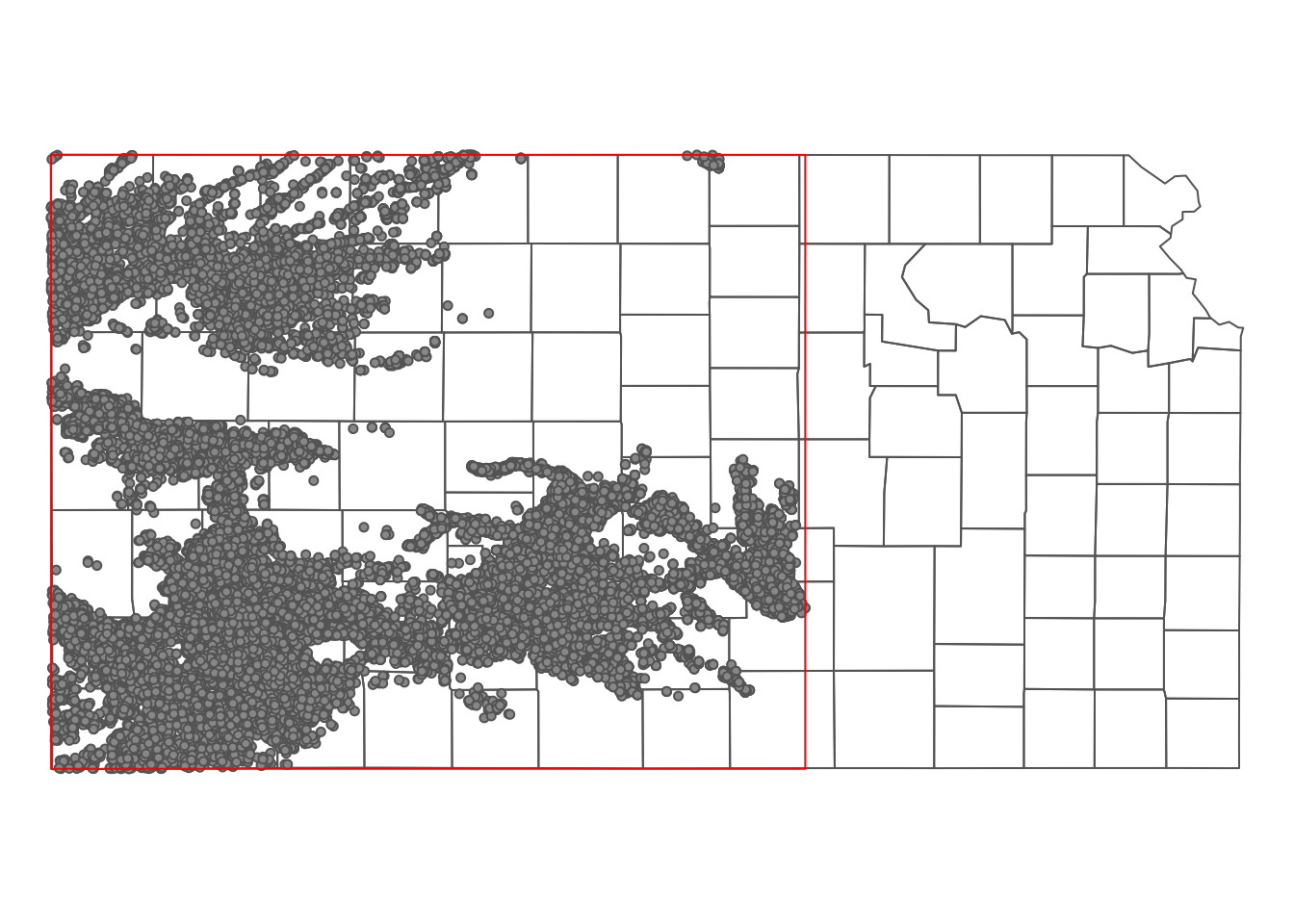
Figure 3.13: The bounding box of the irrigation wells in Kansas that overlie HPA
When you use a bounding box to crop an sf objects, you can consider the bounding box as a single polygon.
Let’s crop KS_counties using the bbox of the irrigation wells.
KS_cropped <- st_crop(KS_counties, bbox_KS_wells_in_hpa) Here is what the cropped data looks like (Figure 3.14):
tm_shape(KS_counties) +
  tm_polygons(col = NA) +
tm_shape(KS_cropped) +
  tm_polygons(col ="blue", alpha = 0.6) +
  tm_layout(frame = NA)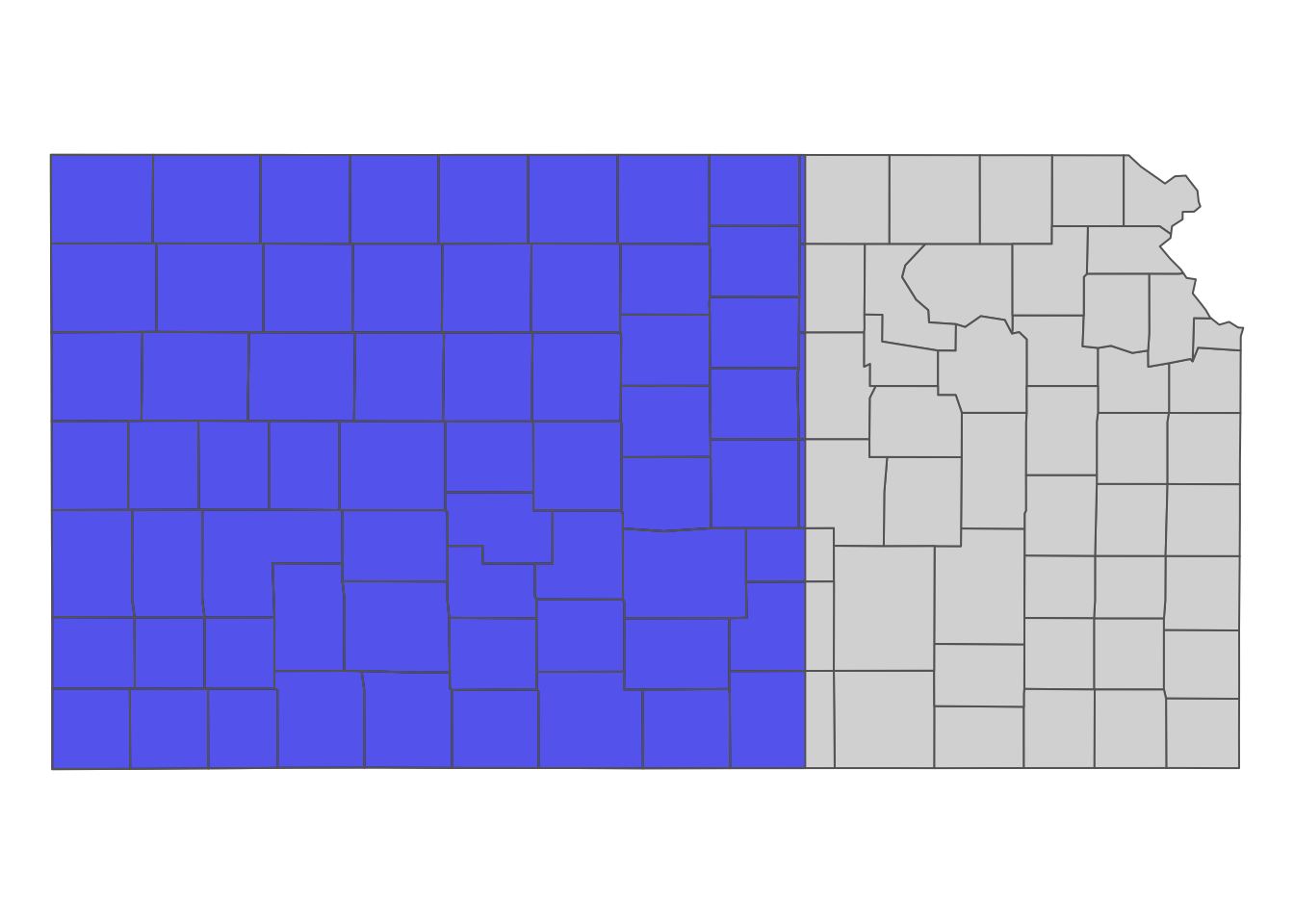
Figure 3.14: The bounding box of the irrigation wells in Kansas that overlie HPA
As you can see, the st_crop() operation cut some counties at the right edge of the bounding box. So, st_crop() is invasive. If you do not like this to happen and want the complete original counties that have at least one well, you can use the subset approach using [, ] after converting the bounding box to an sfc as follows:
KS_complete_counties <- KS_counties[st_as_sfc(bbox_KS_wells_in_hpa), ] Here is what the subsetted Kansas county data looks like (Figure 3.15):
tm_shape(KS_counties) +
  tm_polygons(col = NA) +
tm_shape(KS_complete_counties) +
  tm_polygons(col ="blue", alpha = 0.6) +
  tm_layout(frame = NA)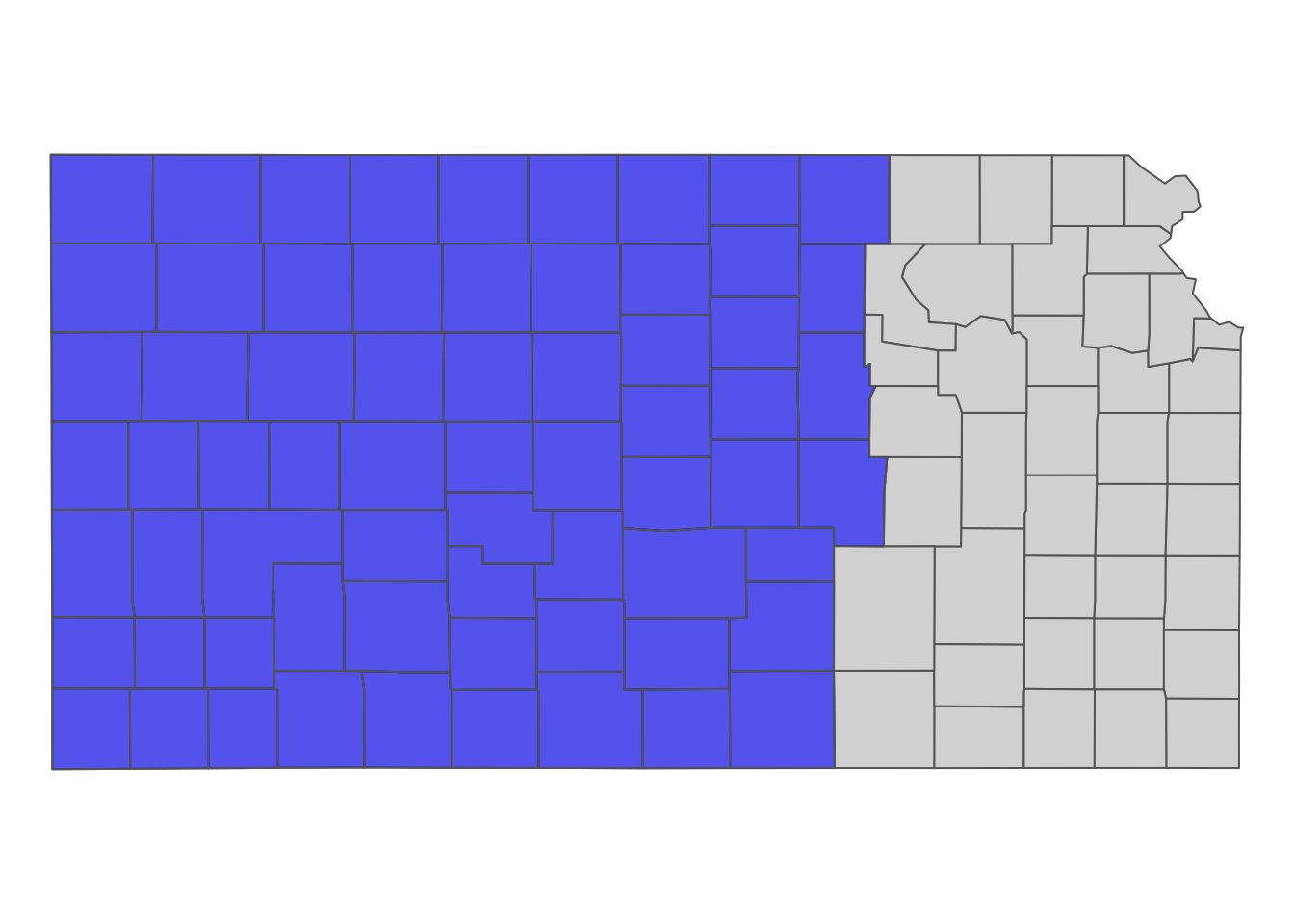
Figure 3.15: The bounding box of the irrigation wells in Kansas that overlie HPA
Notice the difference between the result of this operation and the case where we used KS_wells_in_hpa directly to subset KS_counties as shown in Figure 3.12. The current approach includes counties that do not have any irrigation wells inside them.
If you are a Windows user, you may find that only the
KS_countiesare shown on the created map. There seems to be a limitation to graphics in Windows. See here.↩︎Of course, this situation arises for a polygons-polygons case as well. The above polygons-polygons example was an exception because
hpahad only one polygon object.↩︎