2.1 Spatial Data Structure
Here we learn how the sf package stores spatial data along with the definition of three key sf object classes: simple feature geometry (sfg), simple feature geometry list-column (sfc), and simple feature (sf). The sf package provides a simply way of storing geographic information and the attributes of the geographic units in a single dataset. This special type of dataset is called simple feature (sf). It is best to take a look at an example to see how this is achieved. We use North Carolina county boundaries with county attributes (Figure 2.1).
#--- a dataset that comes with the sf package ---#
nc <- st_read(system.file("shape/nc.shp", package = "sf"))
Reading layer `nc' from data source
`/Library/Frameworks/R.framework/Versions/4.1/Resources/library/sf/shape/nc.shp'
using driver `ESRI Shapefile'
Simple feature collection with 100 features and 14 fields
Geometry type: MULTIPOLYGON
Dimension: XY
Bounding box: xmin: -84.32385 ymin: 33.88199 xmax: -75.45698 ymax: 36.58965
Geodetic CRS: NAD27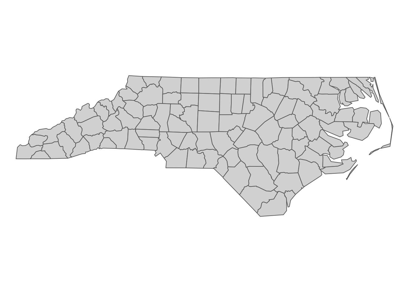
Figure 2.1: North Carolina county boundary
As you can see below, this dataset is of class sf (and data.frame at the same time).
class(nc)[1] "sf" "data.frame"Now, let’s take a look inside of nc.
#--- take a look at the data ---#
head(nc)
Simple feature collection with 6 features and 14 fields
Geometry type: MULTIPOLYGON
Dimension: XY
Bounding box: xmin: -81.74107 ymin: 36.07282 xmax: -75.77316 ymax: 36.58965
Geodetic CRS: NAD27
AREA PERIMETER CNTY_ CNTY_ID NAME FIPS FIPSNO CRESS_ID BIR74 SID74
1 0.114 1.442 1825 1825 Ashe 37009 37009 5 1091 1
2 0.061 1.231 1827 1827 Alleghany 37005 37005 3 487 0
3 0.143 1.630 1828 1828 Surry 37171 37171 86 3188 5
4 0.070 2.968 1831 1831 Currituck 37053 37053 27 508 1
5 0.153 2.206 1832 1832 Northampton 37131 37131 66 1421 9
6 0.097 1.670 1833 1833 Hertford 37091 37091 46 1452 7
NWBIR74 BIR79 SID79 NWBIR79 geometry
1 10 1364 0 19 MULTIPOLYGON (((-81.47276 3...
2 10 542 3 12 MULTIPOLYGON (((-81.23989 3...
3 208 3616 6 260 MULTIPOLYGON (((-80.45634 3...
4 123 830 2 145 MULTIPOLYGON (((-76.00897 3...
5 1066 1606 3 1197 MULTIPOLYGON (((-77.21767 3...
6 954 1838 5 1237 MULTIPOLYGON (((-76.74506 3...Just like a regular data.frame, you see a number of variables (attributes) except that you have a variable called geometry at the end. Each row represents a single geographic unit (here, county). Ashe County (1st row) has area of \(0.114\), FIPS code of \(37009\), and so on. And the entry in geometry column at the first row represents the geographic information of Ashe County. An entry in the geometry column is a simple feature geometry (sfg), which is an \(R\) object that represents the geographic information of a single geometric feature (county in this example). There are different types of sfgs (POINT, LINESTRING, POLYGON, MULTIPOLYGON, etc). Here, sfgs representing counties in NC are of type MULTIPOLYGON. Let’s take a look inside the sfg for Ashe County using st_geometry().
st_geometry(nc[1, ])[[1]][[1]][[1]]
[,1] [,2]
[1,] -81.47276 36.23436
[2,] -81.54084 36.27251
[3,] -81.56198 36.27359
[4,] -81.63306 36.34069
[5,] -81.74107 36.39178
[6,] -81.69828 36.47178
[7,] -81.70280 36.51934
[8,] -81.67000 36.58965
[9,] -81.34530 36.57286
[10,] -81.34754 36.53791
[11,] -81.32478 36.51368
[12,] -81.31332 36.48070
[13,] -81.26624 36.43721
[14,] -81.26284 36.40504
[15,] -81.24069 36.37942
[16,] -81.23989 36.36536
[17,] -81.26424 36.35241
[18,] -81.32899 36.36350
[19,] -81.36137 36.35316
[20,] -81.36569 36.33905
[21,] -81.35413 36.29972
[22,] -81.36745 36.27870
[23,] -81.40639 36.28505
[24,] -81.41233 36.26729
[25,] -81.43104 36.26072
[26,] -81.45289 36.23959
[27,] -81.47276 36.23436As you can see, the sfg consists of a number of points (pairs of two numbers). Connecting the points in the order they are stored delineates the Ashe County boundary.
plot(st_geometry(nc[1, ]))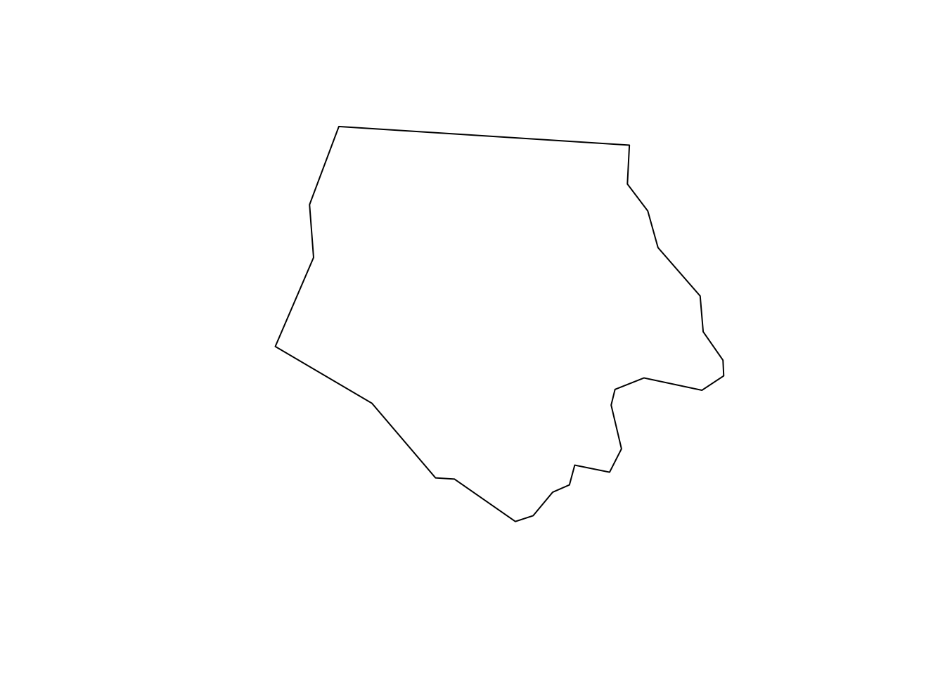
We will take a closer look at different types of sfg in the next section.
Finally, the geometry variable is a list of individual sfgs, called simple feature geometry list-column (sfc).
dplyr::select(nc, geometry)Simple feature collection with 100 features and 0 fields
Geometry type: MULTIPOLYGON
Dimension: XY
Bounding box: xmin: -84.32385 ymin: 33.88199 xmax: -75.45698 ymax: 36.58965
Geodetic CRS: NAD27
First 10 features:
geometry
1 MULTIPOLYGON (((-81.47276 3...
2 MULTIPOLYGON (((-81.23989 3...
3 MULTIPOLYGON (((-80.45634 3...
4 MULTIPOLYGON (((-76.00897 3...
5 MULTIPOLYGON (((-77.21767 3...
6 MULTIPOLYGON (((-76.74506 3...
7 MULTIPOLYGON (((-76.00897 3...
8 MULTIPOLYGON (((-76.56251 3...
9 MULTIPOLYGON (((-78.30876 3...
10 MULTIPOLYGON (((-80.02567 3...Elements of a geometry list-column are allowed to be different in nature from other elements33. In the nc data, all the elements (sfgs) in geometry column are MULTIPOLYGON. However, you could also have LINESTRING or POINT objects mixed with MULTIPOLYGONS objects in a single sf object if you would like.
This is just like a regular
listobject that can contain mixed types of elements: numeric, character, etc↩︎