4 Raster Data Handling
Before you start
In this chapter, we will learn how to use the raster and terra package to handle raster data. The raster package has been the most popular and commonly used package for raster data handling. However, we are in the period of transitioning from the raster package to the terra package. The terra package has been under active development to replace the raster package (see the most up-to-date version of the package here). terra is written in C++ and thus is faster than the raster package in many raster data operations. The raster and terra packages share the same function name for many of the raster operations. Key differences will be discussed and will become clear later.
For economists, raster data extraction for vector data will be by far the most common use case of raster data and also the most time-consuming part of the whole raster data handling experience. Therefore, we will introduce only the essential knowledge of raster data operation required to effectively implement the task of extracting values, which will be covered extensively in Chapter 5. For example, we do not cover raster arithmetic, focal operations, or aggregation. Those who are interested in a fuller treatment of the raster or terra package are referred to Spatial Data Science with R and “terra” or Chapters 3, 4, and 5 of Geocomputation with R, respectively.
Even though the terra package is a replacement of the raster package and it has been out on CRAN for more than several years, we still learn the raster object classes defined by the raster package and how to switch between the raster and terra object classes. This is because other useful packages for us economists were written to work with the raster object classes and have still not been adapted to support terra object classes at the moment.
Finally, you might benefit from learning the stars package for raster data operations (covered in Chapter 7), particularly if you often work with raster data with the temporal dimension (e.g., PRISM, Daymet). It provides a data model that makes working with raster data with temporal dimensions easier. It also allows you to apply dplyr verbs for data wrangling.
Direction for replication
Datasets
All the datasets that you need to import are available here. In this chapter, the path to files is set relative to my own working directory (which is hidden). To run the codes without having to mess with paths to the files, follow these steps:
- set a folder (any folder) as the working directory using
setwd()
- create a folder called “Data” inside the folder designated as the working directory (if you have created a “Data” folder previously, skip this step)
- download the pertinent datasets from here
- place all the files in the downloaded folder in the “Data” folder
Packages
Run the following code to install or load (if already installed) the pacman package, and then install or load (if already installed) the listed package inside the pacman::p_load() function.
if (!require("pacman")) install.packages("pacman")
pacman::p_load(
  terra, # handle raster data
  raster, # handle raster data
  cdlTools, # download CDL data
  mapview, # create interactive maps
  dplyr, # data wrangling
  sf # vector data handling
)
4.1 Raster data object classes
4.1.1 raster package: RasterLayer, RasterStack, and RasterBrick
Let’s start with taking a look at raster data. We will use the CDL data for Iowa in 2015.
class      : RasterLayer
dimensions : 11671, 17795, 207685445  (nrow, ncol, ncell)
resolution : 30, 30  (x, y)
extent     : -52095, 481755, 1938165, 2288295  (xmin, xmax, ymin, ymax)
crs        : +proj=aea +lat_0=23 +lon_0=-96 +lat_1=29.5 +lat_2=45.5 +x_0=0 +y_0=0 +datum=NAD83 +units=m +no_defs
source     : IA_cdl_2015.tif
names      : IA_cdl_2015
values     : 0, 229  (min, max)
Evaluating the imported raster object provides you with information about the raster data, such as dimensions (number of cells, number of columns, number of cells), spatial resolution (30 meter by 30 meter for this raster data), extent, CRS and the minimum and maximum values recorded in this raster layer. The class of the downloaded data is RasterLayer, which is a raster data class defined by the raster package. A RasterLayer consists of only one layer, meaning that only a single variable is associated with the cells (here it is land use category code in integer).
You can stack multiple raster layers of the same spatial resolution and extent to create a RasterStack using raster::stack() or RasterBrick using raster::brick(). Often times, processing a multi-layer object has computational advantages over processing multiple single-layer one by one72.
To create a RasterStack and RasterBrick, let’s load the CDL data for IA in 2016 and stack it with the 2015 data.
class      : RasterStack
dimensions : 11671, 17795, 207685445, 2  (nrow, ncol, ncell, nlayers)
resolution : 30, 30  (x, y)
extent     : -52095, 481755, 1938165, 2288295  (xmin, xmax, ymin, ymax)
crs        : +proj=aea +lat_0=23 +lon_0=-96 +lat_1=29.5 +lat_2=45.5 +x_0=0 +y_0=0 +datum=NAD83 +units=m +no_defs
names      : IA_cdl_2015, IA_cdl_2016
min values :           0,           0
max values :         229,         241
IA_cdl_stack is of class RasterStack, and it has two layers of variables: CDL for 2015 and 2016. You can make it a RasterBrick using raster::brick():
#--- stack the two ---#
IA_cdl_brick <- brick(IA_cdl_stack)

#--- or this works as well ---#
# IA_cdl_brick <- brick(IA_cdl_2015, IA_cdl_2016)

#--- take a look ---#
IA_cdl_brick
You probably noticed that it took some time to create the RasterBrick object73. While spatial operations on RasterBrick are supposedly faster than RasterStack, the time to create a RasterBrick object itself is often long enough to kill the speed advantage entirely74. Often, the three raster object types are collectively referred to as Raster\(^*\) objects for shorthand in the documentation of the raster and other related packages.
4.1.2 terra package: SpatRaster
terra package has only one object class for raster data, SpatRaster and no distinctions between one-layer and multi-layer rasters is necessary. Let’s first convert a RasterLayer to a SpatRaster using terra::rast() function.
#--- convert to a SpatRaster ---#
IA_cdl_2015_sr <- rast(IA_cdl_2015)

#--- take a look ---#
IA_cdl_2015_sr
class : SpatRaster
dimensions : 11671, 17795, 1 (nrow, ncol, nlyr)
resolution : 30, 30 (x, y)
extent : -52095, 481755, 1938165, 2288295 (xmin, xmax, ymin, ymax)
coord. ref. : +proj=aea +lat_0=23 +lon_0=-96 +lat_1=29.5 +lat_2=45.5 +x_0=0 +y_0=0 +datum=NAD83 +units=m +no_defs
source : IA_cdl_2015.tif
color table : 1
name : IA_cdl_2015
min value : 0
max value : 229 You can see that the number of layers (nlyr in dimensions) is \(1\) because the original object is a RasterLayer, which by definition has only one layer. Now, let’s convert a RasterStack to a SpatRaster using terra::rast().
#--- convert to a SpatRaster ---#
IA_cdl_stack_sr <- rast(IA_cdl_stack)

#--- take a look ---#
IA_cdl_stack_sr
class : SpatRaster
dimensions : 11671, 17795, 2 (nrow, ncol, nlyr)
resolution : 30, 30 (x, y)
extent : -52095, 481755, 1938165, 2288295 (xmin, xmax, ymin, ymax)
coord. ref. : +proj=aea +lat_0=23 +lon_0=-96 +lat_1=29.5 +lat_2=45.5 +x_0=0 +y_0=0 +datum=NAD83 +units=m +no_defs
sources : IA_cdl_2015.tif
IA_cdl_2016.tif
color table : 1, 2
names : IA_cdl_2015, IA_cdl_2016
min values : 0, 0
max values : 229, 241 Again, it is a SpatRaster, and you now see that the number of layers is 2. We just confirmed that terra has only one class for raster data whether it is single-layer or multiple-layer ones.
In order to make multi-layer SpatRaster from multiple single-layer SpatRaster you can just use c() like below:
#--- create a single-layer SpatRaster ---#
IA_cdl_2016_sr <- rast(IA_cdl_2016)

#--- concatenate ---#
(
  IA_cdl_ml_sr <- c(IA_cdl_2015_sr, IA_cdl_2016_sr)
)
(
  IA_cdl_ml_sr <- c(IA_cdl_2015_sr, IA_cdl_2016_sr)
)
class : SpatRaster
dimensions : 11671, 17795, 2 (nrow, ncol, nlyr)
resolution : 30, 30 (x, y)
extent : -52095, 481755, 1938165, 2288295 (xmin, xmax, ymin, ymax)
coord. ref. : +proj=aea +lat_0=23 +lon_0=-96 +lat_1=29.5 +lat_2=45.5 +x_0=0 +y_0=0 +datum=NAD83 +units=m +no_defs
sources : IA_cdl_2015.tif
IA_cdl_2016.tif
color table : 1, 2
names : IA_cdl_2015, IA_cdl_2016
min values : 0, 0
max values : 229, 241
4.1.3 Converting a SpatRaster object to a Raster\(^*\) object.
You can convert a SpatRaster object to a Raster\(^*\) object using raster(), stack(), and brick(). Keep in mind that if you use rater() even though SpatRaster has multiple layers, the resulting RasterLayer object has only the first of the multiple layers.
#--- RasterLayer (only 1st layer) ---#
IA_cdl_stack_sr %>% raster()
class : RasterLayer
dimensions : 11671, 17795, 207685445 (nrow, ncol, ncell)
resolution : 30, 30 (x, y)
extent : -52095, 481755, 1938165, 2288295 (xmin, xmax, ymin, ymax)
crs : +proj=aea +lat_0=23 +lon_0=-96 +lat_1=29.5 +lat_2=45.5 +x_0=0 +y_0=0 +datum=NAD83 +units=m +no_defs
source : IA_cdl_2015.tif
names : IA_cdl_2015
values : 0, 229 (min, max)
#--- RasterLayer ---#
IA_cdl_stack_sr %>% stack()
class : RasterStack
dimensions : 11671, 17795, 207685445, 2 (nrow, ncol, ncell, nlayers)
resolution : 30, 30 (x, y)
extent : -52095, 481755, 1938165, 2288295 (xmin, xmax, ymin, ymax)
crs : +proj=aea +lat_0=23 +lon_0=-96 +lat_1=29.5 +lat_2=45.5 +x_0=0 +y_0=0 +datum=NAD83 +units=m +no_defs
names : IA_cdl_2015, IA_cdl_2016
min values : 0, 0
max values : 229, 241
#--- RasterLayer (this takes some time) ---#
IA_cdl_stack_sr %>% brick()
class : RasterStack
dimensions : 11671, 17795, 207685445, 2 (nrow, ncol, ncell, nlayers)
resolution : 30, 30 (x, y)
extent : -52095, 481755, 1938165, 2288295 (xmin, xmax, ymin, ymax)
crs : +proj=aea +lat_0=23 +lon_0=-96 +lat_1=29.5 +lat_2=45.5 +x_0=0 +y_0=0 +datum=NAD83 +units=m +no_defs
names : IA_cdl_2015, IA_cdl_2016
min values : 0, 0
max values : 229, 241 Or, you can just use as(SpatRast, "Raster") like below:
as(IA_cdl_stack_sr, "Raster")class : RasterStack
dimensions : 11671, 17795, 207685445, 2 (nrow, ncol, ncell, nlayers)
resolution : 30, 30 (x, y)
extent : -52095, 481755, 1938165, 2288295 (xmin, xmax, ymin, ymax)
crs : +proj=aea +lat_0=23 +lon_0=-96 +lat_1=29.5 +lat_2=45.5 +x_0=0 +y_0=0 +datum=NAD83 +units=m +no_defs
names : IA_cdl_2015, IA_cdl_2016
min values : 0, 0
max values : 229, 241 This works for any Raster\(^*\) object and you do not have to pick the right function like above.
4.1.4 Vector data in the terra package
terra package has its own class for vector data, called SpatVector. While we do not use any of the vector data functionality provided by the terra package, we learn how to convert an sf object to SpatVector because some of the terra functions do not support sf as of now (this will likely be resolved very soon). We will see some use cases of this conversion in the next chapter when we learn raster value extractions for vector data using terra::extract().
As an example, let’s use Illinois county border data.
Simple feature collection with 102 features and 17 fields
Geometry type: MULTIPOLYGON
Dimension:     XY
Bounding box:  xmin: -91.51308 ymin: 36.9703 xmax: -87.01994 ymax: 42.50848
Geodetic CRS:  NAD83
First 10 features:
    STATEFP COUNTYFP COUNTYNS GEOID    NAME       NAMELSAD LSAD CLASSFP MTFCC
86       17      067 00424235 17067 Hancock Hancock County   06      H1 G4020
92       17      025 00424214 17025    Clay    Clay County   06      H1 G4020
131      17      185 00424293 17185  Wabash  Wabash County   06      H1 G4020
148      17      113 01784833 17113  McLean  McLean County   06      H1 G4020
158      17      005 00424204 17005    Bond    Bond County   06      H1 G4020
159      17      009 00424206 17009   Brown   Brown County   06      H1 G4020
213      17      083 00424243 17083  Jersey  Jersey County   06      H1 G4020
254      17      147 00424275 17147   Piatt   Piatt County   06      H1 G4020
266      17      151 00424277 17151    Pope    Pope County   06      H1 G4020
303      17      011 00424207 17011  Bureau  Bureau County   06      H1 G4020
    CSAFP CBSAFP METDIVFP FUNCSTAT      ALAND   AWATER    INTPTLAT     INTPTLON
86   <NA>   <NA>     <NA>        A 2055798714 53563360 +40.4013180 -091.1688008
92   <NA>   <NA>     <NA>        A 1213023041  3064499 +38.7468187 -088.4823254
131  <NA>   <NA>     <NA>        A  578403995 10973569 +38.4458209 -087.8391674
148  <NA>   <NA>     <NA>        A 3064597288  7804856 +40.4945594 -088.8445391
158  <NA>   <NA>     <NA>        A  985066648  6462629 +38.8859240 -089.4365916
159  <NA>   <NA>     <NA>        A  791828626  4144346 +39.9620694 -090.7503095
213  <NA>   <NA>     <NA>        A  957143527 20333974 +39.0801945 -090.3613850
254  <NA>   <NA>     <NA>        A 1137492088   754122 +40.0090327 -088.5923546
266  <NA>   <NA>     <NA>        A  955362036 14662240 +37.4171687 -088.5423737
303  <NA>   <NA>     <NA>        A 2250884573 11523903 +41.4013043 -089.5283772
                          geometry
86  MULTIPOLYGON (((-90.90609 4...
92  MULTIPOLYGON (((-88.69516 3...
131 MULTIPOLYGON (((-87.89243 3...
148 MULTIPOLYGON (((-88.91954 4...
158 MULTIPOLYGON (((-89.37207 3...
159 MULTIPOLYGON (((-90.53674 3...
213 MULTIPOLYGON (((-90.1459 39...
254 MULTIPOLYGON (((-88.46335 4...
266 MULTIPOLYGON (((-88.48289 3...
303 MULTIPOLYGON (((-89.16654 4...
You can convert an sf object to SpatVector object using terra::vect().
(
  IL_county_sv <- vect(IL_county)
)
class : SpatVector
geometry : polygons
dimensions : 102, 17 (geometries, attributes)
extent : -91.51308, -87.01994, 36.9703, 42.50848 (xmin, xmax, ymin, ymax)
coord. ref. : lon/lat NAD83 (EPSG:4269)
names : STATEFP COUNTYFP COUNTYNS GEOID NAME NAMELSAD LSAD
type : <chr> <chr> <chr> <chr> <chr> <chr> <chr>
values : 17 067 00424235 17067 Hancock Hancock County 06
17 025 00424214 17025 Clay Clay County 06
17 185 00424293 17185 Wabash Wabash County 06
CLASSFP MTFCC CSAFP (and 7 more)
<chr> <chr> <chr>
H1 G4020 NA
H1 G4020 NA
H1 G4020 NA 4.2 Read and write a raster data file
Sometimes we can download raster data of interest as we saw in Section 3.1. But, most of the time you need to read raster data stored as a file. Raster data files can come in numerous different formats. For example, PRPISM comes in the Band Interleaved by Line (BIL) format, some of the Daymet data comes in netCDF format. Other popular formats include GeoTiff, SAGA, ENVI, and many others.
4.2.1 Read raster file(s)
You use terra::rast() to read raster data of many common formats, and it should be almost always the case that the raster data you got can be read using this function. Here, we read a GeoTiff file (a file with .tif extension):
(
  IA_cdl_2015_sr <- rast("Data/IA_cdl_2015.tif")
)
class : SpatRaster
dimensions : 11671, 17795, 1 (nrow, ncol, nlyr)
resolution : 30, 30 (x, y)
extent : -52095, 481755, 1938165, 2288295 (xmin, xmax, ymin, ymax)
coord. ref. : +proj=aea +lat_0=23 +lon_0=-96 +lat_1=29.5 +lat_2=45.5 +x_0=0 +y_0=0 +datum=NAD83 +units=m +no_defs
source : IA_cdl_2015.tif
color table : 1
name : IA_cdl_2015
min value : 0
max value : 229 One important thing to note here is that the cell values of the raster data are actually not in memory when you “read” raster data from a file.
You basically just established a connection to the file. This helps to reduce the memory footprint of raster data handling. You can check this by raster::inMemory() function for Raster\(^*\) objects, but the same function has not been implemented for terra yet.
You can read multiple single-layer raster datasets of the same spatial extent and resolution at the same time to have a multi-layer SpatRaster object. Here, we import two single-layer raster datasets (IA_cdl_2015.tif and IA_cdl_2016.tif) to create a two-layer SpatRaster object.
#--- the list of path to the files ---#
files_list <- c("Data/IA_cdl_2015.tif", "Data/IA_cdl_2016.tif")

#--- read the two at the same time ---#
(
  multi_layer_sr <- rast(files_list)
)
class : SpatRaster
dimensions : 11671, 17795, 2 (nrow, ncol, nlyr)
resolution : 30, 30 (x, y)
extent : -52095, 481755, 1938165, 2288295 (xmin, xmax, ymin, ymax)
coord. ref. : +proj=aea +lat_0=23 +lon_0=-96 +lat_1=29.5 +lat_2=45.5 +x_0=0 +y_0=0 +datum=NAD83 +units=m +no_defs
sources : IA_cdl_2015.tif
IA_cdl_2016.tif
color table : 1, 2
names : IA_cdl_2015, IA_cdl_2016
min values : 0, 0
max values : 229, 241 Of course, this only works because the two datasets have the identical spatial extent and resolution. There are, however, no restrictions on what variable each of the raster layers represent. For example, you can combine PRISM temperature and precipitation raster layers.
4.2.2 Write raster files
You can write a SpatRaster object using terra::writeRaster().
terra::writeRaster(IA_cdl_2015_sr, "Data/IA_cdl_stack.tif", filetype = "GTiff", overwrite = TRUE)The above code saves IA_cdl_2015_sr (a SpatRaster object) as a GeoTiff file.75 The filetype option can be dropped as writeRaster() infers the filetype from the extension of the file name. The overwrite = TRUE option is necessary if a file with the same name already exists and you are overwriting it. This is one of the many areas terra is better than raster. raster::writeRaster() can be frustratingly slow for a large Raster\(^*\) object. terra::writeRaster() is much faster.
You can also save a multi-layer SpatRaster object just like you save a single-layer SpatRaster object.
terra::writeRaster(IA_cdl_stack_sr, "Data/IA_cdl_stack.tif", filetype = "GTiff", overwrite = TRUE)The saved file is a multi-band raster datasets. So, if you have many raster files of the same spatial extent and resolution, you can “stack” them on R and then export it to a single multi-band raster datasets, which cleans up your data folder.
4.3 Extract information from raster data object
4.3.1 Get CRS
You often need to extract the CRS of a raster object before you interact it with vector data (e.g., extracting values from a raster layer to vector data, or cropping a raster layer to the spatial extent of vector data), which can be done using terra::crs():
terra::crs(IA_cdl_2015_sr)[1] "PROJCRS[\"unnamed\",\n BASEGEOGCRS[\"NAD83\",\n DATUM[\"North American Datum 1983\",\n ELLIPSOID[\"GRS 1980\",6378137,298.257222101004,\n LENGTHUNIT[\"metre\",1]]],\n PRIMEM[\"Greenwich\",0,\n ANGLEUNIT[\"degree\",0.0174532925199433]],\n ID[\"EPSG\",4269]],\n CONVERSION[\"Albers Equal Area\",\n METHOD[\"Albers Equal Area\",\n ID[\"EPSG\",9822]],\n PARAMETER[\"Latitude of false origin\",23,\n ANGLEUNIT[\"degree\",0.0174532925199433],\n ID[\"EPSG\",8821]],\n PARAMETER[\"Longitude of false origin\",-96,\n ANGLEUNIT[\"degree\",0.0174532925199433],\n ID[\"EPSG\",8822]],\n PARAMETER[\"Latitude of 1st standard parallel\",29.5,\n ANGLEUNIT[\"degree\",0.0174532925199433],\n ID[\"EPSG\",8823]],\n PARAMETER[\"Latitude of 2nd standard parallel\",45.5,\n ANGLEUNIT[\"degree\",0.0174532925199433],\n ID[\"EPSG\",8824]],\n PARAMETER[\"Easting at false origin\",0,\n LENGTHUNIT[\"metre\",1],\n ID[\"EPSG\",8826]],\n PARAMETER[\"Northing at false origin\",0,\n LENGTHUNIT[\"metre\",1],\n ID[\"EPSG\",8827]]],\n CS[Cartesian,2],\n AXIS[\"easting\",east,\n ORDER[1],\n LENGTHUNIT[\"metre\",1,\n ID[\"EPSG\",9001]]],\n AXIS[\"northing\",north,\n ORDER[2],\n LENGTHUNIT[\"metre\",1,\n ID[\"EPSG\",9001]]]]"4.3.2 Subset
You can access specific layers in a multi-layer raster object by indexing:
#--- index ---#
IA_cdl_stack_sr[[2]] # (originally IA_cdl_2016.tif)
class : SpatRaster
dimensions : 11671, 17795, 1 (nrow, ncol, nlyr)
resolution : 30, 30 (x, y)
extent : -52095, 481755, 1938165, 2288295 (xmin, xmax, ymin, ymax)
coord. ref. : +proj=aea +lat_0=23 +lon_0=-96 +lat_1=29.5 +lat_2=45.5 +x_0=0 +y_0=0 +datum=NAD83 +units=m +no_defs
source : IA_cdl_2016.tif
color table : 1
name : IA_cdl_2016
min value : 0
max value : 241 4.3.3 Get cell values
You can access the values stored in a SpatRaster object using the terra::values() function:
#--- terra::values ---#
values_from_rs <- terra::values(IA_cdl_stack_sr)

#--- take a look ---#
head(values_from_rs)
Layer_1 Layer_1
[1,] 0 0
[2,] 0 0
[3,] 0 0
[4,] 0 0
[5,] 0 0
[6,] 0 0The returned values come in a matrix form of two columns because we are getting values from a two-layer SpatRaster object (one column for each layer). In general, terra::values() returns a \(X\) by \(n\) matrix, where \(X\) is the number of cells and \(n\) is the number of layers.
4.4 Turning a raster object into a data.frame
When creating maps using ggplot2() from a SpatRaster or Raster\(^*\) object, it is necessary to first convert it to a data.frame (see Chapter 8.2). You can use the as.data.frame() function with xy = TRUE option to construct a data.frame where each row represents a single cell that has cell values for each layer and its coordinates (the center of the cell).
#--- converting to a data.frame ---#
IA_cdl_df <- as.data.frame(IA_cdl_stack_sr, xy = TRUE) # this works with Raster* objects as well

#--- take a look ---#
head(IA_cdl_df)
x y Layer_1 Layer_1.1
1 -52080 2288280 0 0
2 -52050 2288280 0 0
3 -52020 2288280 0 0
4 -51990 2288280 0 0
5 -51960 2288280 0 0
6 -51930 2288280 0 0 Note: I have seen cases where a raster object is converted to a data.frame and then to ‘sf’ for the purpose of interacting it with polygons using st_join() to extract and assign cell values for the polygons (see Chapter 3 for this type of operation). This is, however, not generally recommended for two reasons. First of all, it is much slower than using functions that work on a raster object and polygons directly to extract values for the polygons, such as terra::extract() or exactextractr::exact_extract(), which are introduced in Chapter 5. This is primarily because converting a raster object to a data.frame() is very slow. Second, once a raster data object is converted to a point sf data, one can no longer weight cell values according to the degree of their overlaps with the target polygons. The only case I have found the conversion beneficial (or simply necessary) is to create a map using ggplot() from a raster object (the tmap package can work directly with raster objects.). While the desire to work with a data.frame is understandable as we are very comfortable with working on a data.frame, it is very likely that the conversion to a data.frame is not only unnecessary, but also inefficient76.
4.5 Quick visualization
To have a quick visualization of the data values of SpatRaster objects, you can simply use plot():
plot(IA_cdl_2015_sr)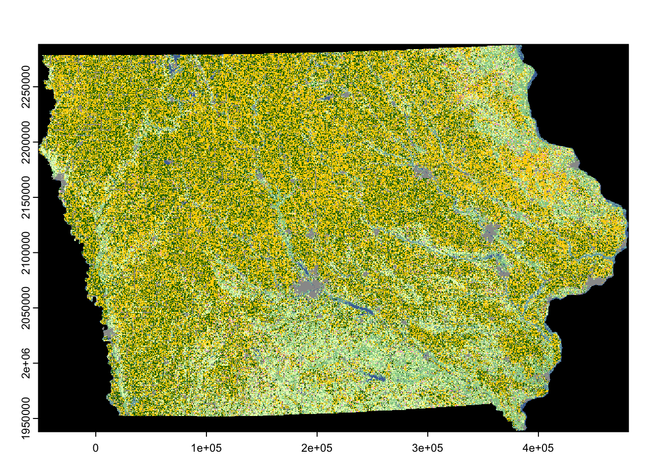
For a more elaborate map using raster data, see Chapter 8.2.
4.6 Working with netCDFs
It is worth talking about how to read a netCDFs format – a multidimensional file format that resembles a raster stack/brick. A netCDF file contains data with a specific structure: a two-dimensional spatial grid (e.g., longitude and latitude) and a third dimension which is usually date or time. This structure is convenient for weather data measured on a consistent grid over time. One such dataset is called gridMET which maintains a gridded dataset of weather variables at 4km resolution. Let’s download the daily precipitation data for 2018 using downloader::download()77. We set the destination file name (what to call the file and where we want it to be), and the mode to wb for a binary download.
#--- download gridMET precipitation 2018 ---#
downloader::download(
  url = str_c("http://www.northwestknowledge.net/metdata/data/pr_2018.nc"),
  destfile = "Data/pr_2018.nc",
  mode = "wb"
)
This code should have stored the data as pr_2018.nc in the Data folder. You can read a netCDF file using terra::rast().
(
  pr_2018_gm <- rast("Data/pr_2018.nc")
)
class : SpatRaster
dimensions : 585, 1386, 365 (nrow, ncol, nlyr)
resolution : 0.04166667, 0.04166667 (x, y)
extent : -124.7875, -67.0375, 25.04583, 49.42083 (xmin, xmax, ymin, ymax)
coord. ref. : lon/lat WGS 84 (EPSG:4326)
source : pr_2018.nc
varname : precipitation_amount (pr)
names : preci~43099, preci~43100, preci~43101, preci~43102, preci~43103, preci~43104, ...
unit : mm, mm, mm, mm, mm, mm, ... You can see that it has 365 layers: one layer per day in 2018. Let’s now look at layer names:
[1] "precipitation_amount_day=43099" "precipitation_amount_day=43100"
[3] "precipitation_amount_day=43101" "precipitation_amount_day=43102"
[5] "precipitation_amount_day=43103" "precipitation_amount_day=43104"
Since we have 365 layers and the number at the end of the layer names increase by 1, you would think that nth layer represents nth day of 2018. In this case, you are correct. However, it is always a good practice to confirm what each layer represents without assuming anything. Now, let’s use the ncdf4 package, which is built specifically to handle netCDF4 objects.
(
  pr_2018_nc <- ncdf4::nc_open("Data/pr_2018.nc")
)
File Data/pr_2018.nc (NC_FORMAT_NETCDF4):
1 variables (excluding dimension variables):
unsigned short precipitation_amount[lon,lat,day] (Chunking: [231,98,61]) (Compression: level 9)
_FillValue: 32767
units: mm
description: Daily Accumulated Precipitation
long_name: pr
standard_name: pr
missing_value: 32767
dimensions: lon lat time
grid_mapping: crs
coordinate_system: WGS84,EPSG:4326
scale_factor: 0.1
add_offset: 0
coordinates: lon lat
_Unsigned: true
4 dimensions:
lon Size:1386
units: degrees_east
description: longitude
long_name: longitude
standard_name: longitude
axis: X
lat Size:585
units: degrees_north
description: latitude
long_name: latitude
standard_name: latitude
axis: Y
day Size:365
description: days since 1900-01-01
units: days since 1900-01-01 00:00:00
long_name: time
standard_name: time
calendar: gregorian
crs Size:1
grid_mapping_name: latitude_longitude
longitude_of_prime_meridian: 0
semi_major_axis: 6378137
long_name: WGS 84
inverse_flattening: 298.257223563
GeoTransform: -124.7666666333333 0.041666666666666 0 49.400000000000000 -0.041666666666666
spatial_ref: GEOGCS["WGS 84",DATUM["WGS_1984",SPHEROID["WGS 84",6378137,298.257223563,AUTHORITY["EPSG","7030"]],AUTHORITY["EPSG","6326"]],PRIMEM["Greenwich",0,AUTHORITY["EPSG","8901"]],UNIT["degree",0.0174532925199433,AUTHORITY["EPSG","9122"]],AUTHORITY["EPSG","4326"]]
19 global attributes:
geospatial_bounds_crs: EPSG:4326
Conventions: CF-1.6
geospatial_bounds: POLYGON((-124.7666666333333 49.400000000000000, -124.7666666333333 25.066666666666666, -67.058333300000015 25.066666666666666, -67.058333300000015 49.400000000000000, -124.7666666333333 49.400000000000000))
geospatial_lat_min: 25.066666666666666
geospatial_lat_max: 49.40000000000000
geospatial_lon_min: -124.7666666333333
geospatial_lon_max: -67.058333300000015
geospatial_lon_resolution: 0.041666666666666
geospatial_lat_resolution: 0.041666666666666
geospatial_lat_units: decimal_degrees north
geospatial_lon_units: decimal_degrees east
coordinate_system: EPSG:4326
author: John Abatzoglou - University of Idaho, jabatzoglou@uidaho.edu
date: 03 May 2021
note1: The projection information for this file is: GCS WGS 1984.
note2: Citation: Abatzoglou, J.T., 2013, Development of gridded surface meteorological data for ecological applications and modeling, International Journal of Climatology, DOI: 10.1002/joc.3413
note3: Data in slices after last_permanent_slice (1-based) are considered provisional and subject to change with subsequent updates
note4: Data in slices after last_provisional_slice (1-based) are considered early and subject to change with subsequent updates
note5: Days correspond approximately to calendar days ending at midnight, Mountain Standard Time (7 UTC the next calendar day)As you can see from the output, there is tons of information that we did not see when we read the data using rast(), which includes the explanation of the third dimension (day) of this raster object. It turned out that the numerical values at the end of layer names in the SpatRaster object are days since 1900-01-01. So, the first layer (named precipitation_amount_day=43099) represents:
ymd("1900-01-01") + 43099[1] "2018-01-01"Actually, if we use raster::brick(), instead of terra::rast(), then we can see the naming convention of the layers:
(
  pr_2018_b <- brick("Data/pr_2018.nc")
)
class : RasterBrick
dimensions : 585, 1386, 810810, 365 (nrow, ncol, ncell, nlayers)
resolution : 0.04166667, 0.04166667 (x, y)
extent : -124.7875, -67.0375, 25.04583, 49.42083 (xmin, xmax, ymin, ymax)
crs : +proj=longlat +datum=WGS84 +no_defs
source : pr_2018.nc
names : X43099, X43100, X43101, X43102, X43103, X43104, X43105, X43106, X43107, X43108, X43109, X43110, X43111, X43112, X43113, ...
day (days since 1900-01-01 00:00:00): 43099, 43463 (min, max)
varname : precipitation_amount SpatRaster or RasterBrick objects are easier to work with as many useful functions accept them as inputs, but not the ncdf4 object. Personally, I first scrutinize a netCDFs file using nc_open() and then import it as a SpatRaster or RasterBrick object78. Recovering the dates for the layers is particularly important as we often wrangle the resulting data based on date (e.g., subset the data so that you have only April to September). An example of date recovery can be seen in Chapter 9.5.
Very detailed description of how to work with ncdf4 object is provided here. However, I would say that economists are unlikely to benefit much from it. As I have stated several times already, we (economists) rarely need to manipulate raster data itself. Our observation units are almost always points (e.g., farms, houses) or polygons (e.g., county boundary) and we just need to associate those units with the values held in raster data (e.g., precipitation). We can simply use raster objects as they are and supply them to functions that take care of the business of raster value extraction, which is covered in the next chapter (Chapter 5).