9 Download and process spatial datasets from within R
Before you start
There are many publicly available spatial datasets that can be downloaded using R. Programming data downloading using R instead of manually downloading data from websites can save lots of time and also enhances the reproducibility of your analysis. In this section, we will introduce some of such datasets and show how to download and process those data.
Direction for replication
Datasets
No datasets to download for this Chapter.
Packages
- Run the following code to install or load (if already installed) the
pacmanpackage, and then install or load (if already installed) the listed package inside thepacman::p_load()function.
if (!require("pacman")) install.packages("pacman")
pacman::p_load(
  stars, # spatiotemporal data handling
  terra, # raster data handling
  raster, # raster data handling
  sf, # vector data handling
  dplyr, # data wrangling
  stringr, # string manipulation
  lubridate, # dates handling
  data.table, # data wrangling
  tidyr, # reshape
  tidyUSDA, # download USDA NASS data
  keyring, # API key management
  FedData, # download Daymet data
  daymetr, # download Daymet data
  ggplot2, # make maps
  tmap, # make maps
  future.apply, # parallel processing
  CropScapeR, # download CDL data
  prism, # download PRISM data
  exactextractr # extract raster values to sf
)- Run the following code to define the theme for map:
theme_set(theme_bw())

theme_for_map <- theme(
  axis.ticks = element_blank(),
  axis.text = element_blank(),
  axis.line = element_blank(),
  panel.border = element_blank(),
  panel.grid.major = element_line(color = "transparent"),
  panel.grid.minor = element_line(color = "transparent"),
  panel.background = element_blank(),
  plot.background = element_rect(fill = "transparent", color = "transparent")
)
9.1 USDA NASS QuickStat with tidyUSDA
There are several packages that lets you download data from the USDA NASS QuickStat. Here we use the tidyUSDA package (Lindblad 2020). A nice thing about tidyUSDA is that it gives you an option to download data as an sf object, which means you can immediately visualize the data or spatially interact it with other spatial objects.
First thing you want to do is to get an API key from this website, which you need to actually download data.
You can download data using getQuickstat(). There are number of options you can use to narrow down the scope of the data you are downloading including data_item, geographic_level, year, commodity, and so on. See its manual for the full list of parameters you can set. As an example, the code below download corn-related data by county in Illinois for year 2016 as an sf object.
(
  IL_corn_yield <-
    getQuickstat(
      #--- put your API key in place of key_get("usda_nass_qs_api") ---#
      key = key_get("usda_nass_qs_api"),
      program = "SURVEY",
      commodity = "CORN",
      geographic_level = "COUNTY",
      state = "ILLINOIS",
      year = "2016",
      geometry = TRUE
    ) %>%
    #--- keep only some of the variables ---#
    dplyr::select(
      year, county_name, county_code, state_name,
      state_fips_code, short_desc, Value
    )
)
Simple feature collection with 384 features and 7 fields (with 16 geometries empty)
Geometry type: MULTIPOLYGON
Dimension: XY
Bounding box: xmin: -91.51308 ymin: 36.9703 xmax: -87.01993 ymax: 42.50848
Geodetic CRS: NAD83
First 10 features:
year county_name county_code state_name state_fips_code short_desc
1 2016 BUREAU 011 ILLINOIS 17 CORN - ACRES PLANTED
2 2016 CARROLL 015 ILLINOIS 17 CORN - ACRES PLANTED
3 2016 HENRY 073 ILLINOIS 17 CORN - ACRES PLANTED
4 2016 JO DAVIESS 085 ILLINOIS 17 CORN - ACRES PLANTED
5 2016 LEE 103 ILLINOIS 17 CORN - ACRES PLANTED
6 2016 MERCER 131 ILLINOIS 17 CORN - ACRES PLANTED
7 2016 OGLE 141 ILLINOIS 17 CORN - ACRES PLANTED
8 2016 PUTNAM 155 ILLINOIS 17 CORN - ACRES PLANTED
9 2016 ROCK ISLAND 161 ILLINOIS 17 CORN - ACRES PLANTED
10 2016 STEPHENSON 177 ILLINOIS 17 CORN - ACRES PLANTED
Value geometry
1 273500 MULTIPOLYGON (((-89.85691 4...
2 147500 MULTIPOLYGON (((-90.16133 4...
3 235000 MULTIPOLYGON (((-90.43247 4...
4 100500 MULTIPOLYGON (((-90.50668 4...
5 258500 MULTIPOLYGON (((-89.63118 4...
6 142500 MULTIPOLYGON (((-90.99255 4...
7 228000 MULTIPOLYGON (((-89.68598 4...
8 37200 MULTIPOLYGON (((-89.33303 4...
9 65000 MULTIPOLYGON (((-90.33573 4...
10 179500 MULTIPOLYGON (((-89.92577 4...As you can see, it is an sf object with geometry column due to geometry = TRUE option. This means that you can immediately create a map with the data (Figure 9.1):
ggplot() +
  geom_sf(
    data = filter(IL_corn_yield, short_desc == "CORN, GRAIN - YIELD, MEASURED IN BU / ACRE"),
    aes(fill = Value)
  ) +
  theme_for_map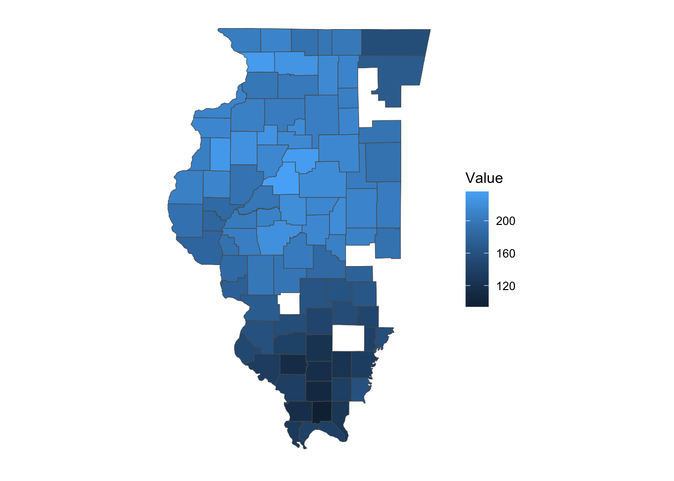
Figure 9.1: Corn Yield (bu/acre) in Illinois in 2016
You can download data for multiple states and years at the same time like below (if you want data for the whole U.S., don’t specify the state parameter).
(
  IL_CO_NE_corn <-
    getQuickstat(
      key = key_get("usda_nass_qs_api"),
      program = "SURVEY",
      commodity = "CORN",
      geographic_level = "COUNTY",
      state = c("ILLINOIS", "COLORADO", "NEBRASKA"),
      year = paste(2014:2018),
      geometry = TRUE
    ) %>%
    #--- keep only some of the variables ---#
    dplyr::select(
      year, county_name, county_code, state_name,
      state_fips_code, short_desc, Value
    )
)
Simple feature collection with 6384 features and 7 fields (with 588 geometries empty)
Geometry type: MULTIPOLYGON
Dimension: XY
Bounding box: xmin: -109.0459 ymin: 36.9703 xmax: -87.01993 ymax: 43.00171
Geodetic CRS: NAD83
First 10 features:
year county_name county_code state_name state_fips_code
1 2018 OTHER (COMBINED) COUNTIES 998 COLORADO 08
2 2017 OTHER (COMBINED) COUNTIES 998 COLORADO 08
3 2016 OTHER (COMBINED) COUNTIES 998 COLORADO 08
4 2015 OTHER (COMBINED) COUNTIES 998 COLORADO 08
5 2014 OTHER (COMBINED) COUNTIES 998 COLORADO 08
6 2017 BOULDER 013 COLORADO 08
7 2016 BOULDER 013 COLORADO 08
8 2016 LARIMER 069 COLORADO 08
9 2015 LARIMER 069 COLORADO 08
10 2014 LARIMER 069 COLORADO 08
short_desc Value geometry
1 CORN - ACRES PLANTED 107600 MULTIPOLYGON EMPTY
2 CORN - ACRES PLANTED 108900 MULTIPOLYGON EMPTY
3 CORN - ACRES PLANTED 163600 MULTIPOLYGON EMPTY
4 CORN - ACRES PLANTED 3100 MULTIPOLYGON EMPTY
5 CORN - ACRES PLANTED 5200 MULTIPOLYGON EMPTY
6 CORN - ACRES PLANTED 3000 MULTIPOLYGON (((-105.6486 4...
7 CORN - ACRES PLANTED 3300 MULTIPOLYGON (((-105.6486 4...
8 CORN - ACRES PLANTED 12800 MULTIPOLYGON (((-105.8225 4...
9 CORN - ACRES PLANTED 14900 MULTIPOLYGON (((-105.8225 4...
10 CORN - ACRES PLANTED 13600 MULTIPOLYGON (((-105.8225 4...9.1.1 Look for parameter values
This package has a function that lets you see all the possible parameter values you can use for many of these parameters. For example, suppose you know you would like irrigated corn yields in Colorado, but you are not sure what parameter value (string) you should supply to the data_item parameter. Then, you can do this:95
#--- get all the possible values for data_item ---#
all_items <- tidyUSDA::allDataItem

#--- take a look at the first six ---#
head(all_items)
short_desc1
"AG LAND - ACRES"
short_desc2
"AG LAND - NUMBER OF OPERATIONS"
short_desc3
"AG LAND - OPERATIONS WITH TREATED"
short_desc4
"AG LAND - TREATED, MEASURED IN ACRES"
short_desc5
"AG LAND, (EXCL CROPLAND & PASTURELAND & WOODLAND) - ACRES"
short_desc6
"AG LAND, (EXCL CROPLAND & PASTURELAND & WOODLAND) - AREA, MEASURED IN PCT OF AG LAND" You can use key words like “CORN”, “YIELD”, “IRRIGATED” to narrow the entire list using grep()96:
all_items %>%
  grep(pattern = "CORN", ., value = TRUE) %>%
  grep(pattern = "YIELD", ., value = TRUE) %>%
  grep(pattern = "IRRIGATED", ., value = TRUE)
short_desc9227
"CORN, GRAIN, IRRIGATED - YIELD, MEASURED IN BU / ACRE"
short_desc9228
"CORN, GRAIN, IRRIGATED - YIELD, MEASURED IN BU / NET PLANTED ACRE"
short_desc9233
"CORN, GRAIN, IRRIGATED, ENTIRE CROP - YIELD, MEASURED IN BU / ACRE"
short_desc9236
"CORN, GRAIN, IRRIGATED, NONE OF CROP - YIELD, MEASURED IN BU / ACRE"
short_desc9238
"CORN, GRAIN, IRRIGATED, PART OF CROP - YIELD, MEASURED IN BU / ACRE"
short_desc9249
"CORN, GRAIN, NON-IRRIGATED - YIELD, MEASURED IN BU / ACRE"
short_desc9250
"CORN, GRAIN, NON-IRRIGATED - YIELD, MEASURED IN BU / NET PLANTED ACRE"
short_desc9291
"CORN, SILAGE, IRRIGATED - YIELD, MEASURED IN TONS / ACRE"
short_desc9296
"CORN, SILAGE, IRRIGATED, ENTIRE CROP - YIELD, MEASURED IN TONS / ACRE"
short_desc9299
"CORN, SILAGE, IRRIGATED, NONE OF CROP - YIELD, MEASURED IN TONS / ACRE"
short_desc9301
"CORN, SILAGE, IRRIGATED, PART OF CROP - YIELD, MEASURED IN TONS / ACRE"
short_desc9307
"CORN, SILAGE, NON-IRRIGATED - YIELD, MEASURED IN TONS / ACRE"
short_desc28557
"SWEET CORN, IRRIGATED - YIELD, MEASURED IN CWT / ACRE"
short_desc28564
"SWEET CORN, NON-IRRIGATED - YIELD, MEASURED IN CWT / ACRE" Looking at the list, we know the exact text value we want, which is the first entry of the vector.
(
  CO_ir_corn_yield <-
    getQuickstat(
      key = key_get("usda_nass_qs_api"),
      program = "SURVEY",
      data_item = "CORN, GRAIN, IRRIGATED - YIELD, MEASURED IN BU / ACRE",
      geographic_level = "COUNTY",
      state = "COLORADO",
      year = "2018",
      geometry = TRUE
    ) %>%
    #--- keep only some of the variables ---#
    dplyr::select(year, NAME, county_code, short_desc, Value)
)
Here is the complete list of functions that gives you the possible values of the parameters for getQuickstat().
tidyUSDA::allCategory
tidyUSDA::allSector
tidyUSDA::allGroup
tidyUSDA::allCommodity
tidyUSDA::allDomain
tidyUSDA::allCounty
tidyUSDA::allProgram
tidyUSDA::allDataItem
tidyUSDA::allState
tidyUSDA::allGeogLevel
9.1.2 Caveats
You cannot retrieve more than \(50,000\) (the limit is set by QuickStat) rows of data. The query below requests much more than \(50,000\) observations, and fail. In this case, you need to narrow the search and chop the task into smaller tasks.
many_states_corn <- getQuickstat(
  key = key_get("usda_nass_qs_api"),
  program = "SURVEY",
  commodity = "CORN",
  geographic_level = "COUNTY",
  state = c("ILLINOIS", "COLORADO", "NEBRASKA", "IOWA", "KANSAS"),
  year = paste(1995:2018),
  geometry = TRUE
)
Error: API did not return results. First verify that your input parameters work on the NASS
website: https://quickstats.nass.usda.gov/. If correct, try again in a few minutes; the API may
be experiencing heavy traffic.Another caveat is that the query returns an error when there is no observation that satisfy your query criteria. For example, even though “CORN, GRAIN, IRRIGATED - YIELD, MEASURED IN BU / ACRE” is one of the values you can use for data_item, there is no entry for the statistic in Illinois in 2018. Therefore, the following query fails.
many_states_corn <-
  getQuickstat(
    key = key_get("usda_nass_qs_api"),
    program = "SURVEY",
    data_item = "CORN, GRAIN, IRRIGATED - YIELD, MEASURED IN BU / ACRE",
    geographic_level = "COUNTY",
    state = "ILLINOIS",
    year = "2018",
    geometry = TRUE
  )
Error: API did not return results. First verify that your input parameters work on the NASS
website: https://quickstats.nass.usda.gov/. If correct, try again in a few minutes; the API may
be experiencing heavy traffic.
9.2 CDL with CropScapeR
The Cropland Data Layer (CDL) is a data product produced by the National Agricultural Statistics Service of U.S. Department of Agriculture. CDL provides geo-referenced, high accuracy, 30 (after 2007) or 56 (in 2006 and 2007) meter resolution, crop-specific cropland land cover information for up to 48 contiguous states in the U.S. from 1997 to the present. This data product has been extensively used in agricultural research. CropScape is an interactive Web CDL exploring system (https://nassgeodata.gmu.edu/CropScape/), and it was developed to query, visualize, disseminate, and analyze CDL data geospatially through standard geospatial web services in a publicly accessible on-line environment (Han et al., 2012).
This section shows how to use the CropScapeR package (Chen 2020) to download and explore the CDL data. The package implements some of the most useful geospatial processing services provided by the CropScape, and it allows users to efficiently process the CDL data within the R environment. Specifically, the CropScapeR package provides four functions that implement different kinds of geospatial processing services provided by the CropScape. This section introduces these functions while providing some examples. GetCDLData() in particular is the most important function as it lets you download the raw CDL data. The other functions provide the users with the CDL data summarized or transformed in particular manners that may suit the need of some users.
Note: There is a known problem with Mac users requesting CDL data services using the CropScape API, which causes errors when using the functions provided by the package. Please see section 9.2.4 for a workaround.
The CropScapeR package can be installed directly from ‘CRAN’:
install.packages("CropScapeR")The development version of the package can be downloaded from its GitHub website using the following codes:
library(devtools)
devtools::install_github("cbw1243/CropScapeR")
Let’s load the package.
library(CropScapeR)Acknowledgment: The development of the CropScapeR package was supported by USDA-NRCS Agreement No. NR193A750016C001 through the Cooperative Ecosystem Studies Units network. Any opinions, findings, conclusions, or recommendations expressed are those of the author(s) and do not necessarily reflect the view of the U.S. Department of Agriculture.
9.2.1 GetCDLData: Download the CDL data as raster data
GetCDLData() allows us to obtain CDL data for any Area of Interest (AOI) in a given year. It requires three parameters to make a valid data request:
-
aoi: Area of Interest (AOI).
-
year: Year of the data to request.
-
type: Type of AOI.
The following AOI-type combinations are accepted:
- any spatial object as an
sforsfcobject -type = "b" - county (defined by a 5-digit county FIPS code) -
type = "f" - state (defined by a 2-digit state FIPS code) -
type = "f" - bounding box (defined by four corner points) -
type = "b" - polygon area (defined by at least three coordinates) -
type = "ps" - single point (defined by a coordinate) -
type = "p"
This section discusses how to download data for an sf object, county, and state as they are likely to be the most common AOI. See the package github site (https://github.com/cbw1243/CropScapeR) to see how the other options work.
9.2.1.1 Downloading CDL data for sf, county, and state
Downloading CDL data for sf
Let’s download the 2018 CDL data for the area that covers Champaign, Vermilion, Ford, and Iroquois Counties in Illinois (a map below).
#--- get the sf for the four counties  ---#
IL_4_county <-
  tigris::counties(state = "IL", cb = TRUE) %>%
  st_as_sf() %>%
  filter(NAME %in% c("Champaign", "Vermilion", "Ford", "Iroquois"))
ggplot() +
  geom_sf(data = IL_county) +
  geom_sf(data = IL_county_4, fill = "lightblue") +
  theme_void()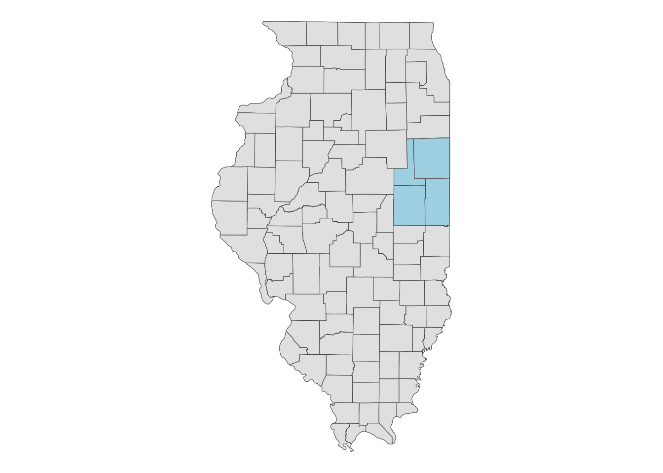
When you use an sf object for aoi, CDL data will be downloaded for the bounding box (this is why type = "b") that encompasses the entire geographic area of the sf object irrespective of the type of objects in the sf object (whether they are points, polygons, lines). In this case, CDL data is downloaded for the red area in the map below.
ggplot() +
  geom_sf(data = IL_county) +
  geom_sf(data = st_as_sfc(st_bbox(IL_county_4)), fill = "red", alpha = 0.4) +
  theme_void()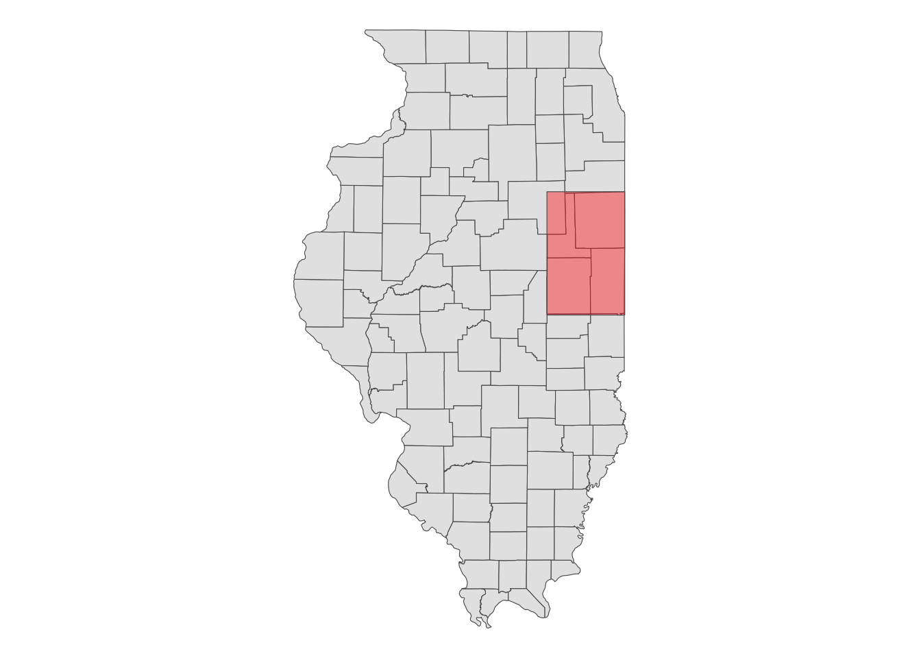
Let’s download CDL data for the four counties:
(
  cdl_IL_4 <-
    GetCDLData(
      aoi = IL_county_4,
      year = "2018",
      type = "b"
    )
)
class : RasterLayer
dimensions : 4431, 2826, 12522006 (nrow, ncol, ncell)
resolution : 30, 30 (x, y)
extent : 631935, 716715, 1898745, 2031675 (xmin, xmax, ymin, ymax)
crs : +proj=aea +lat_0=23 +lon_0=-96 +lat_1=29.5 +lat_2=45.5 +x_0=0 +y_0=0 +datum=NAD83 +units=m +no_defs
source : IL4.tif
names : Layer_1 As you can see, the downloaded data is a RasterLayer object97. Note that the CDL data uses the Albers equal-area conic projection.
terra::crs(cdl_IL_4)Coordinate Reference System:
Deprecated Proj.4 representation:
+proj=aea +lat_0=23 +lon_0=-96 +lat_1=29.5 +lat_2=45.5 +x_0=0 +y_0=0
+datum=NAD83 +units=m +no_defs
WKT2 2019 representation:
PROJCRS["unknown",
BASEGEOGCRS["unknown",
DATUM["North American Datum 1983",
ELLIPSOID["GRS 1980",6378137,298.257222101,
LENGTHUNIT["metre",1]],
ID["EPSG",6269]],
PRIMEM["Greenwich",0,
ANGLEUNIT["degree",0.0174532925199433],
ID["EPSG",8901]]],
CONVERSION["unknown",
METHOD["Albers Equal Area",
ID["EPSG",9822]],
PARAMETER["Latitude of false origin",23,
ANGLEUNIT["degree",0.0174532925199433],
ID["EPSG",8821]],
PARAMETER["Longitude of false origin",-96,
ANGLEUNIT["degree",0.0174532925199433],
ID["EPSG",8822]],
PARAMETER["Latitude of 1st standard parallel",29.5,
ANGLEUNIT["degree",0.0174532925199433],
ID["EPSG",8823]],
PARAMETER["Latitude of 2nd standard parallel",45.5,
ANGLEUNIT["degree",0.0174532925199433],
ID["EPSG",8824]],
PARAMETER["Easting at false origin",0,
LENGTHUNIT["metre",1],
ID["EPSG",8826]],
PARAMETER["Northing at false origin",0,
LENGTHUNIT["metre",1],
ID["EPSG",8827]]],
CS[Cartesian,2],
AXIS["(E)",east,
ORDER[1],
LENGTHUNIT["metre",1,
ID["EPSG",9001]]],
AXIS["(N)",north,
ORDER[2],
LENGTHUNIT["metre",1,
ID["EPSG",9001]]]] Take a look at the downloaded CDL data.
plot(cdl_IL_4)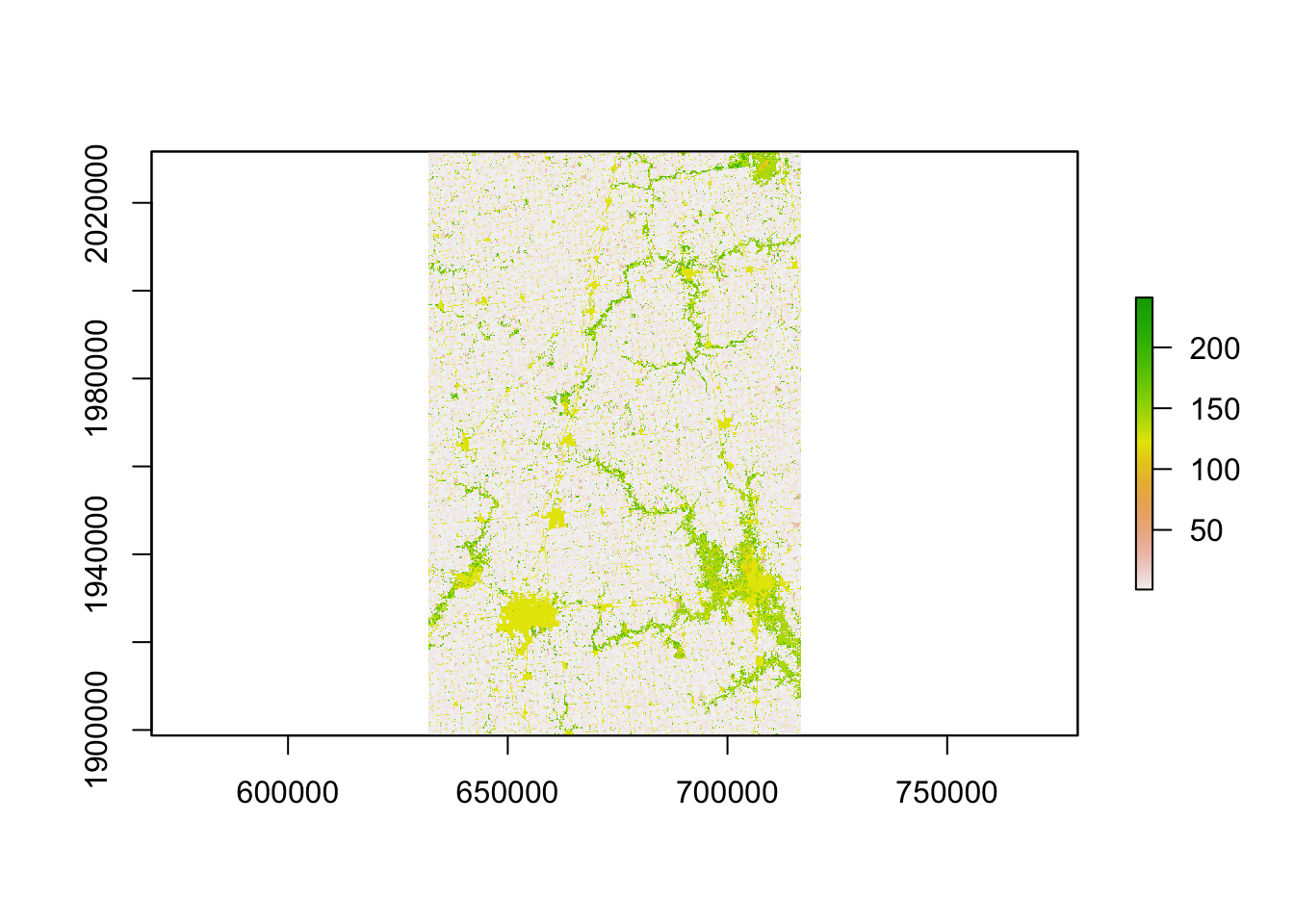
If you do not want to have values outside of the sf object, you can use raster::mask() to turn them into NA as follows:
cdl_IL_4_masked <- IL_county_4 %>%
  #--- change the CRS first to that of the raster data ---#
  st_transform(., projection(cdl_IL_4)) %>%
  #--- mask the values outside the sf (turn them into NA) ---#
  raster::mask(cdl_IL_4, .)
As you can see below, values outside the four counties are now NA (black area):
plot(cdl_IL_4_masked)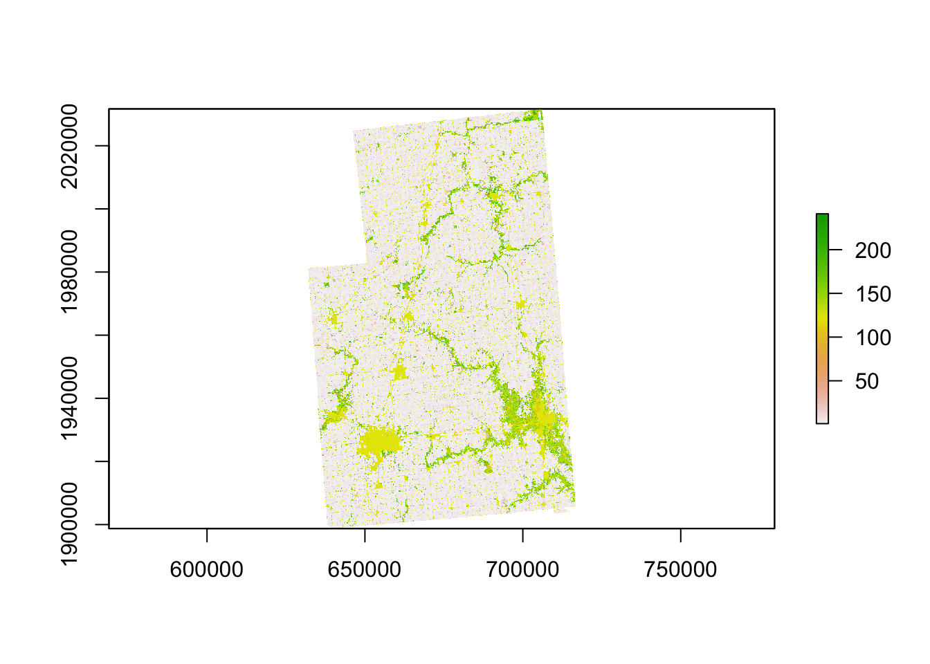
Downloading CDL data for county
The following code makes a request to download the CDL data for Champaign county in Illinois in 2018.
(
  cdl_Champaign <- GetCDLData(aoi = 17019, year = 2018, type = "f")
)
class : RasterLayer
dimensions : 2060, 1626, 3349560 (nrow, ncol, ncell)
resolution : 30, 30 (x, y)
extent : 633825, 682605, 1898745, 1960545 (xmin, xmax, ymin, ymax)
crs : +proj=aea +lat_0=23 +lon_0=-96 +lat_1=29.5 +lat_2=45.5 +x_0=0 +y_0=0 +datum=NAD83 +units=m +no_defs
source : ch.tif
names : Layer_1 In the above code, the FIPS code for Champaign County (17019) was supplied to the aoi option. Because a county is used here, the type argument is specified as ‘f’.
plot(cdl_Champaign)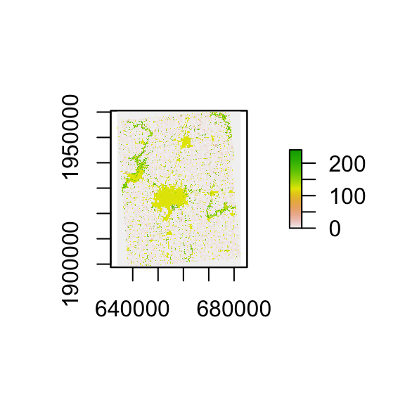
Downloading CDL data for state
The following code makes a request to download the CDL data for the state of Illinois in 2018.
(
  cdl_IL <- GetCDLData(aoi = 17, year = 2018, type = "f")
)
In the above code, the state FIPS code for Illinois (\(17\)) was supplied to the aoi option. Because a county is used here, the type argument is specified as ‘f’.
plot(cdl_IL)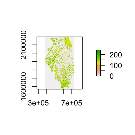
9.2.1.2 Other format options
GeoTiff
You could save the downloaded CDL data as a tif file by adding save_path = option to GetCDLData() as follows:
(
  cdl_IL_4 <- GetCDLData(
    aoi = IL_county_4,
    year = "2018",
    type = "b",
    save_path = "Data/IL_4.tif"
  )
)
With this code, the downloaded data will be saved as “IL_4.tif” in the “Data” folder residing in the current working directory.
sf
The GetCDLData function lets you download CDL data as an sf of points, where the coordinates of the points are the coordinates of the centroid of the raster cells. This can be done by adding format = sf as an option.
(
  cdl_sf <- GetCDLData(aoi = 17019, year = 2018, type = "f", format = "sf")
)
The first column (value) is the crop code. Of course, you can manually convert a RasterLayer to an sf of points as follows:
as.data.frame(cdl_Champaign, xy = TRUE) %>%
  #--- to sf consisting of points ---#
  st_as_sf(coords = c("x", "y")) %>%
  #--- Albert conic projection ---#
  st_set_crs("+proj=aea +lat_1=29.5 +lat_2=45.5 +lat_0=23 +lon_0=-96 +x_0=0 +y_0=0 +ellps=GRS80 +towgs84=0,0,0,0,0,0,0 +units=m +no_defs")
Simple feature collection with 3349560 features and 1 field
Geometry type: POINT
Dimension: XY
Bounding box: xmin: 633840 ymin: 1898760 xmax: 682590 ymax: 1960530
Projected CRS: +proj=aea +lat_1=29.5 +lat_2=45.5 +lat_0=23 +lon_0=-96 +x_0=0 +y_0=0 +ellps=GRS80 +towgs84=0,0,0,0,0,0,0 +units=m +no_defs
First 10 features:
Layer_1 geometry
1 0 POINT (633840 1960530)
2 0 POINT (633870 1960530)
3 0 POINT (633900 1960530)
4 0 POINT (633930 1960530)
5 0 POINT (633960 1960530)
6 0 POINT (633990 1960530)
7 0 POINT (634020 1960530)
8 0 POINT (634050 1960530)
9 0 POINT (634080 1960530)
10 0 POINT (634110 1960530)The format = sf option makes GetCDLData() do this conversion internally for those who want CDL data as an sf consisting of points instead of a RasterLayer.
9.2.2 Data processing after downloading data
The downloaded raster data itself is not readily usable immediately for your economic analysis. Typically the variable of interest is the frequency of land use types or their shares. You can use raster::freq() to get the frequency (the number of raster cells) of each land use type.
(
  crop_freq <- freq(cdl_Champaign)
)
value count
[1,] 0 476477
[2,] 1 1211343
[3,] 4 15
[4,] 5 1173150
[5,] 23 8
[6,] 24 8869
[7,] 26 1168
[8,] 27 34
[9,] 28 52
[10,] 36 4418
[11,] 37 6804
[12,] 43 2
[13,] 59 1064
[14,] 60 79
[15,] 61 54
[16,] 111 6112
[17,] 121 111191
[18,] 122 155744
[19,] 123 38898
[20,] 124 12232
[21,] 131 1333
[22,] 141 49012
[23,] 142 15
[24,] 143 7
[25,] 152 77
[26,] 176 84463
[27,] 190 6545
[28,] 195 339
[29,] 222 1
[30,] 229 16
[31,] 241 38Clearly, once frequencies are found, you can easily get shares as well:
(
  crop_data <- crop_freq %>%
    #--- matrix to data.frame ---#
    data.frame(.) %>%
    #--- find share ---#
    mutate(share = count / sum(count))
)
value count share
1 0 476477 1.422506e-01
2 1 1211343 3.616424e-01
3 4 15 4.478200e-06
4 5 1173150 3.502400e-01
5 23 8 2.388373e-06
6 24 8869 2.647810e-03
7 26 1168 3.487025e-04
8 27 34 1.015059e-05
9 28 52 1.552443e-05
10 36 4418 1.318979e-03
11 37 6804 2.031312e-03
12 43 2 5.970933e-07
13 59 1064 3.176537e-04
14 60 79 2.358519e-05
15 61 54 1.612152e-05
16 111 6112 1.824717e-03
17 121 111191 3.319570e-02
18 122 155744 4.649685e-02
19 123 38898 1.161287e-02
20 124 12232 3.651823e-03
21 131 1333 3.979627e-04
22 141 49012 1.463237e-02
23 142 15 4.478200e-06
24 143 7 2.089827e-06
25 152 77 2.298809e-05
26 176 84463 2.521615e-02
27 190 6545 1.953988e-03
28 195 339 1.012073e-04
29 222 1 2.985467e-07
30 229 16 4.776747e-06
31 241 38 1.134477e-05At this point, the data does not tell you which value corresponds to which crop. To find the crop names associated with the crop codes (value), you can get the reference table using data(linkdata) from the CropScapeR package.98
#--- load the crop code reference data ---#
data("linkdata")
You can merge the two data sets using value from the CDL data and MasterCat from linkdata as the merging keys:
   value   count        share                     Crop
1      0  476477 1.422506e-01                   NoData
2      1 1211343 3.616424e-01                     Corn
3      4      15 4.478200e-06                  Sorghum
4      5 1173150 3.502400e-01                 Soybeans
5     23       8 2.388373e-06             Spring_Wheat
6     24    8869 2.647810e-03             Winter_Wheat
7     26    1168 3.487025e-04 Dbl_Crop_WinWht/Soybeans
8     27      34 1.015059e-05                      Rye
9     28      52 1.552443e-05                     Oats
10    36    4418 1.318979e-03                  Alfalfa
11    37    6804 2.031312e-03    Other_Hay/Non_Alfalfa
12    43       2 5.970933e-07                 Potatoes
13    59    1064 3.176537e-04           Sod/Grass_Seed
14    60      79 2.358519e-05              Switchgrass
15    61      54 1.612152e-05     Fallow/Idle_Cropland
16   111    6112 1.824717e-03               Open_Water
17   121  111191 3.319570e-02     Developed/Open_Space
18   122  155744 4.649685e-02  Developed/Low_Intensity
19   123   38898 1.161287e-02  Developed/Med_Intensity
20   124   12232 3.651823e-03 Developed/High_Intensity
21   131    1333 3.979627e-04                   Barren
22   141   49012 1.463237e-02         Deciduous_Forest
23   142      15 4.478200e-06         Evergreen_Forest
24   143       7 2.089827e-06             Mixed_Forest
25   152      77 2.298809e-05                Shrubland
26   176   84463 2.521615e-02        Grassland/Pasture
27   190    6545 1.953988e-03           Woody_Wetlands
28   195     339 1.012073e-04      Herbaceous_Wetlands
29   222       1 2.985467e-07                   Squash
30   229      16 4.776747e-06                 Pumpkins
31   241      38 1.134477e-05   Dbl_Crop_Corn/Soybeans
NoData in Crop corresponds to the black area in the above figure, which is the portion of the raster data that does not overlap with the boundary of Champaign County. These points with NoData can be removed by using the filter function.
9.2.3 Other forms of CDL data
Instead of downloading the raw CDL data, CropScape provides an option to download summarized CDL data.
-
GetCDLComp: request data on land use changes -
GetCDLStat: get acreage estimates from the CDL -
GetCDLImage: download the image files of the CDL data
These may come handy if they satisfy your needs because you can skip post-downloading processing steps.
GetCDLComp(): request data on land use changes
The GetCDLComp function allows users to request data on changes in land cover over time from the CDL. Specifically, this function returns acres changed from one crop category to another crop category between two years for a user-defined AOI.
Let’s see an example. The following codes request data on acreage changes in land cover for Champaign County (FIPS = 17019) from 2017 (year1 = 2017) to 2018 (year2 = 2018).
(
  data_change <- GetCDLComp(aoi = "17019", year1 = 2017, year2 = 2018, type = "f")
)
From To Count Acreage aoi
<char> <char> <int> <num> <char>
1: Corn Corn 181490 40362.4 17019
2: Corn Sorghum 1 0.2 17019
3: Corn Soybeans 1081442 240506.9 17019
4: Corn Winter Wheat 1950 433.7 17019
5: Corn Dbl Crop WinWht/Soybeans 110 24.5 17019
---
241: Herbaceous Wetlands Herbaceous Wetlands 18 4.0 17019
242: Dbl Crop WinWht/Corn Corn 1 0.2 17019
243: Pumpkins Corn 69 15.3 17019
244: Pumpkins Sorghum 2 0.4 17019
245: Pumpkins Soybeans 62 13.8 17019What is returned is a data.frame (data.table) that has 5 columns. The columns “From” and “To” are crop names. The column “Count” is the pixel count, and “Acreage” is the acres corresponding to the pixel counts. The last column “aoi” is the selected AOI. The first row of the returned data table shows the acreage (i.e., 40,362 acres) of continuous corn during 2017 and 2018. The third row shows the acreage (i.e., 240,506 acres) rotated from corn to soybeans during 2017 and 2018.
Remember that the spatial resolution changes from 56 meters to 30 meters starting 2008. This means that when data is requested for land use changes from 2007 to 2008, two CDL raster layers have different spatial resolutions. Consequently, CropScape API fails to resolve the issue and return an error message saying “Mismatch size of file 1 and file 2.” The GetCDLComp() function manually resolves this problem by resampling two CDL raster files using the nearest neighbor resampling technique such that both rasters have the same spatial resolutions. The finer resolution raster is downscaled to the lower resolution. Then, the resampled raster layers are merged together to calculate cropland changes. Users can turn off this default behavior by adding manual_try = FALSE option. In this case, an error message from CropScape API will be returned with no land use changes results.
data_change <- GetCDLComp(aoi = "17019", year1 = 2007, year2 = 2008, type = "f", `manual_try` = FALSE)Error in GetCDLCompF(fips = aoi, year1 = year1, year2 = year2, mat = mat, : Error: The requested data might not exist in the CDL database.
Error message from CropScape is :<faultstring>Error: Mismatch size of file 1 and file 2.
</faultstring>GetCDLStat(): get acreage estimates from the CDL
The GetCDLStat function allows users to get acreage by land cover category for a user defined AOI in a year. For example, the following codes request data on acreage by land cover categories for Champaign County in Illinois in 2018. You can see that the pixel counts are already converted to acres and category names are attached.
(
  data_stat <- GetCDLStat(aoi = 17019, year = 2018, type = "f")
)
Value Category Acreage
<int> <char> <num>
1: 1 Corn 269396.2
2: 4 Sorghum 3.3
3: 5 Soybeans 260902.3
4: 23 Spring Wheat 1.8
5: 24 Winter Wheat 1972.4
6: 26 Dbl Crop WinWht/Soybeans 259.8
7: 27 Rye 7.6
8: 28 Oats 11.6
9: 36 Alfalfa 982.5
10: 37 Other Hay/Non Alfalfa 1513.2
11: 43 Potatoes 0.4
12: 59 Sod/Grass Seed 236.6
13: 60 Switchgrass 17.6
14: 61 Fallow/Idle Cropland 12.0
15: 111 Open Water 1359.3
16: 121 Developed/Open Space 24728.3
17: 122 Developed/Low Intensity 34636.6
18: 123 Developed/Medium Intensity 8650.7
19: 124 Developed/High Intensity 2720.3
20: 131 Barren 296.5
21: 141 Deciduous Forest 10900.0
22: 142 Evergreen Forest 3.3
23: 143 Mixed Forest 1.6
24: 152 Shrubland 17.1
25: 176 Grass/Pasture 18784.1
26: 190 Woody Wetlands 1455.6
27: 195 Herbaceous Wetlands 75.4
28: 222 Squash 0.2
29: 229 Pumpkins 3.6
30: 241 Dbl Crop Corn/Soybeans 8.5
Value Category AcreageGetCDLImage(): Download the image files of the CDL data
The GetCDLImage function allows users to download the image files of the CDL data. This function is very similar to the GetCDLData function, except that image files are returned. This function can be helpful if you only want to look at the picture of the CDL data. By default, the picture is saved as the ‘png’ format. You can also save it in the ‘kml’ format.
GetCDLImage(aoi = 17019, year = 2018, type = "f", verbose = F)9.2.4 SSL certificate problem on Mac
SSL refers to the Secure Sockets Layer, and SSL certificate displays important information for verifying the owner of a website and encrypting web traffic with SSL/TLS for securing connection. It is a known problem that Mac users encounter the following error when GetCDLData() is used: ‘SSL certificate problem: SSL certificate expired’. As the name suggests, this is because the CropScape server has an expired certificate. While this affects the Mac users, Windows users should not expect this issue.
To avoid the problem for Mac users, the CropScapeR has a workaround that involves downloading the GeoTiff file for the requested AOI first, and then read the file using the raster() function as a RasterLayer.99
You first need to run the following code before requesting data from CDL.
#--- Skip the SSL check ---#
httr::set_config(httr::config(ssl_verifypeer = 0L))
Now, you can download CDL data by specifying the file path with the save_path option like below:
#--- Download the raster TIF file into specified path, also read into R ---#
data <- GetCDLData(aoi = 17019, year = 2018, type = "f", save_path = "Data/ch.tif")
Hopefully, this problem is fixed by the maintainer of CropScape so that this workaround is not necessary for Mac users.
9.3 PRISM with prism
9.3.1 Basics
PRISM dataset provide model-based estimates of precipitation, tmax, and tmin for the U.S. at the 4km by 4km spatial resolution. Here, we use get_prism_dailys() from the prism package (Hart and Bell 2015) to download daily data. Here is its general syntax:
#--- NOT RUN ---#
get_prism_dailys(
  type = variable type,
  minDate = starting date as character,
  maxDate = ending date as character,
  keepZip = TRUE or FALSE
)
The variables types you can select from is “ppt” (precipitation), “tmean” (mean temperature), “tmin” (minimum temperature), and “tmax” (maximum temperature). For minDate and maxDate, the dates must be specified in a specific format of “YYYY-MM-DD”. keepZip = FALSE does not keep the zipped folders of the downloaded files as the name suggests.
Before you download PRISM data using the function, it is recommended that you set the path to folder in which the downloaded PRISM will be stored using options(prism.path = "path"). For example, the following set the path to “Data/PRISM/” relative to the current working directory.
options(prism.path = "Data/PRISM/")The following code downloads daily precipitation data from January 1, 2000 to Jan 10, 2000.
#--- NOT RUN ---#
get_prism_dailys(
  type = "ppt",
  minDate = "2000-01-01",
  maxDate = "2000-01-10",
  keepZip = FALSE
)
When you download data using the above code, you will notice that it creates one folder for one day. For example, for precipitation data for “2000-01-01”, you can get the path to the downloaded file as follows:
var_type <- "ppt" # variable type
dates_prism_txt <- str_remove_all("2000-01-01", "-") # date without dashes

#--- folder name ---#
folder_name <- paste0("PRISM_", var_type, "_stable_4kmD2_", dates_prism_txt, "_bil")

#--- file name of the downloaded data inside the above folder ---#
file_name <- paste0("PRISM_", var_type, "_stable_4kmD2_", dates_prism_txt, "_bil.bil")

#--- path to the file relative to the designated data folder (here, it's "Data/PRISM/") ---#
(
  file_path <- paste0("Data/PRISM/", folder_name, "/", file_name)
)
[1] "Data/PRISM/PRISM_ppt_stable_4kmD2_20000101_bil/PRISM_ppt_stable_4kmD2_20000101_bil.bil"We can then easily read the data using terra::rast() or stars::read_stars() if you prefer the stars way.
#--- as SpatRaster ---#
(
  prism_2000_01_01_sr <- rast(file_path)
)
class : SpatRaster
dimensions : 621, 1405, 1 (nrow, ncol, nlyr)
resolution : 0.04166667, 0.04166667 (x, y)
extent : -125.0208, -66.47917, 24.0625, 49.9375 (xmin, xmax, ymin, ymax)
coord. ref. : lon/lat NAD83
source : PRISM_ppt_stable_4kmD2_20000101_bil.bil
name : PRISM_ppt_stable_4kmD2_20000101_bil
min value : 0.000
max value : 49.848
#--- as stars ---#
(
  prism_2000_01_01_stars <- read_stars(file_path)
)
stars object with 2 dimensions and 1 attribute
attribute(s):
Min. 1st Qu. Median Mean 3rd Qu. Max.
PRISM_ppt_stable_4kmD2_2000... 0 0 0 0.4952114 0 49.848
NA's
PRISM_ppt_stable_4kmD2_2000... 390874
dimension(s):
from to offset delta refsys x/y
x 1 1405 -125 0.04167 NAD83 [x]
y 1 621 49.94 -0.04167 NAD83 [y]Here is a quick visualization of the data (Figure 9.2):
plot(prism_2000_01_01_stars)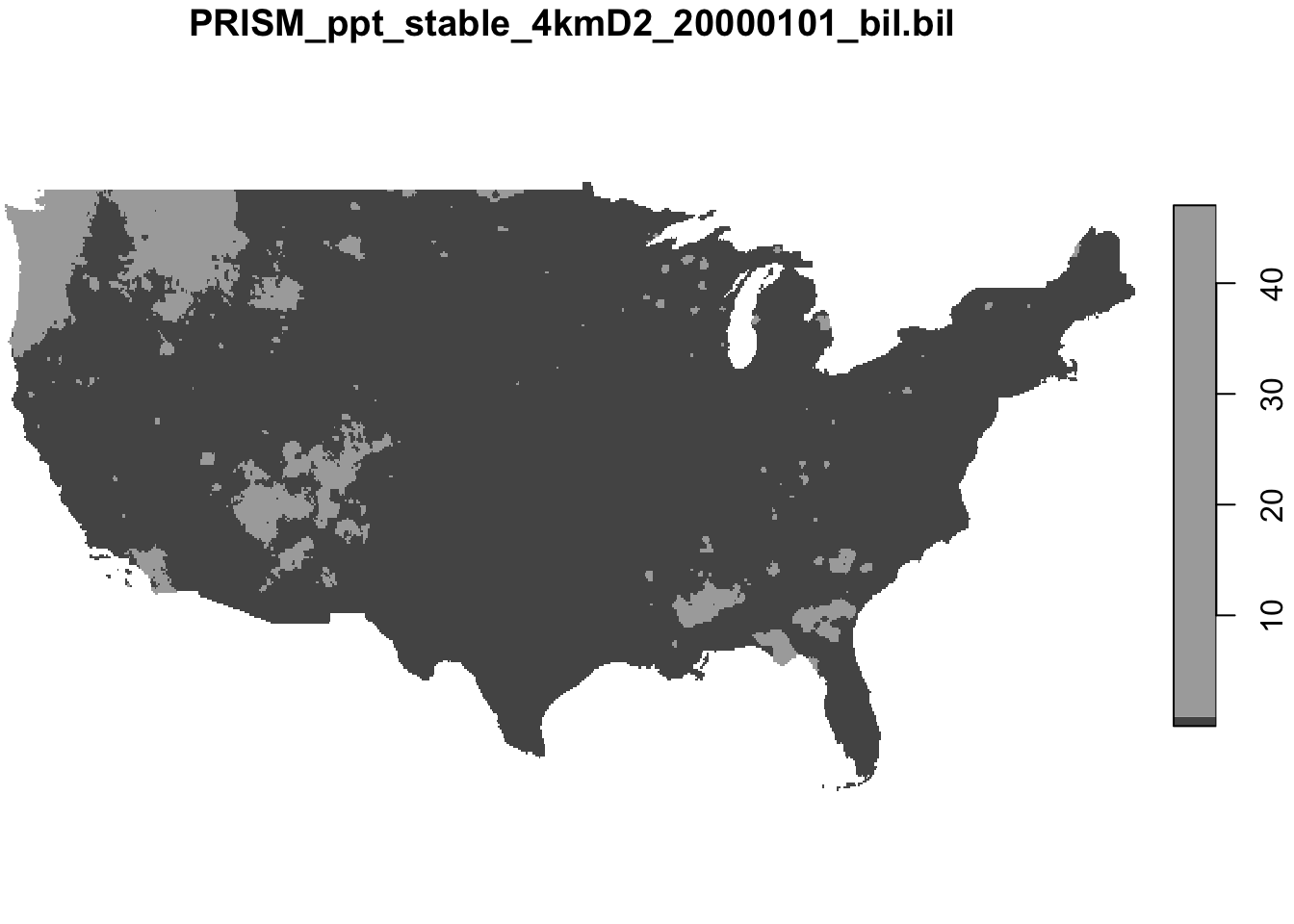
Figure 9.2: PRISM precipitation data for January 1, 2000
As you can see, the data covers the entire contiguous U.S.
9.3.2 Download daily PRISM data for many years and build your own datasets
Here, an example of how to create your own sets of PRISM datasets is presented. Creating such datasets and have them locally can be useful if you expect to use the data for many different projects in the future.
Suppose we are interested in saving daily PRISM precipitation data by year-month from 1980 to 2018. We will write a loop that loops over all the year-month combinations. Before writing a loop, let’s work on the code for a particular year-month combination: 1990-December. However, we will write codes in a way that can be easily translated into a looped operations later. Specifically, we will define the following variables and use them as if they are variables to be looped over in a loop.
#--- month to work on ---#
temp_month <- 12

#--- year to work on ---#
temp_year <- 1990
We first need to set the path to the folder in which daily PRISM files will be downloaded.
#--- set your own path ---#
options(prism.path = "Data/PRISM/")
We then set the start and end dates for get_prism_dailys().
#--- starting date of the working month-year ---#
(
  start_date <- dmy(paste0("1/", temp_month, "/", temp_year))
)
[1] "1990-12-01"
#--- ending date: add a month and then go back 1 day ---#
(
  end_date <- start_date %m+% months(1) - 1
)
[1] "1990-12-31"We now download PRISM data for the year-month we are working on.
#--- download daily PRISM data for the working month-year ---#
get_prism_dailys(
  type = "ppt",
  minDate = as.character(start_date),
  maxDate = as.character(end_date),
  keepZip = FALSE
)
Once all the data are downloaded, we will read and import them onto R. To do so, we will need the path to all the downloaded files.
#--- list of dates of the working month-year ---#
dates_ls <- seq(start_date, end_date, "days")

#--- remove dashes ---#
dates_prism_txt <- str_remove_all(dates_ls, "-")

#--- folder names ---#
folder_name <- paste0("PRISM_", var_type, "_stable_4kmD2_", dates_prism_txt, "_bil")

#--- the file name of the downloaded data ---#
file_name <- paste0("PRISM_", var_type, "_stable_4kmD2_", dates_prism_txt, "_bil.bil")

#--- complete path to the downloaded files ---#
(
  file_path <- paste0("Data/PRISM/", folder_name, "/", file_name)
)
[1] "Data/PRISM/PRISM_ppt_stable_4kmD2_19901201_bil/PRISM_ppt_stable_4kmD2_19901201_bil.bil"
[2] "Data/PRISM/PRISM_ppt_stable_4kmD2_19901202_bil/PRISM_ppt_stable_4kmD2_19901202_bil.bil"
[3] "Data/PRISM/PRISM_ppt_stable_4kmD2_19901203_bil/PRISM_ppt_stable_4kmD2_19901203_bil.bil"
[4] "Data/PRISM/PRISM_ppt_stable_4kmD2_19901204_bil/PRISM_ppt_stable_4kmD2_19901204_bil.bil"
[5] "Data/PRISM/PRISM_ppt_stable_4kmD2_19901205_bil/PRISM_ppt_stable_4kmD2_19901205_bil.bil"
[6] "Data/PRISM/PRISM_ppt_stable_4kmD2_19901206_bil/PRISM_ppt_stable_4kmD2_19901206_bil.bil"
[7] "Data/PRISM/PRISM_ppt_stable_4kmD2_19901207_bil/PRISM_ppt_stable_4kmD2_19901207_bil.bil"
[8] "Data/PRISM/PRISM_ppt_stable_4kmD2_19901208_bil/PRISM_ppt_stable_4kmD2_19901208_bil.bil"
[9] "Data/PRISM/PRISM_ppt_stable_4kmD2_19901209_bil/PRISM_ppt_stable_4kmD2_19901209_bil.bil"
[10] "Data/PRISM/PRISM_ppt_stable_4kmD2_19901210_bil/PRISM_ppt_stable_4kmD2_19901210_bil.bil"
[11] "Data/PRISM/PRISM_ppt_stable_4kmD2_19901211_bil/PRISM_ppt_stable_4kmD2_19901211_bil.bil"
[12] "Data/PRISM/PRISM_ppt_stable_4kmD2_19901212_bil/PRISM_ppt_stable_4kmD2_19901212_bil.bil"
[13] "Data/PRISM/PRISM_ppt_stable_4kmD2_19901213_bil/PRISM_ppt_stable_4kmD2_19901213_bil.bil"
[14] "Data/PRISM/PRISM_ppt_stable_4kmD2_19901214_bil/PRISM_ppt_stable_4kmD2_19901214_bil.bil"
[15] "Data/PRISM/PRISM_ppt_stable_4kmD2_19901215_bil/PRISM_ppt_stable_4kmD2_19901215_bil.bil"
[16] "Data/PRISM/PRISM_ppt_stable_4kmD2_19901216_bil/PRISM_ppt_stable_4kmD2_19901216_bil.bil"
[17] "Data/PRISM/PRISM_ppt_stable_4kmD2_19901217_bil/PRISM_ppt_stable_4kmD2_19901217_bil.bil"
[18] "Data/PRISM/PRISM_ppt_stable_4kmD2_19901218_bil/PRISM_ppt_stable_4kmD2_19901218_bil.bil"
[19] "Data/PRISM/PRISM_ppt_stable_4kmD2_19901219_bil/PRISM_ppt_stable_4kmD2_19901219_bil.bil"
[20] "Data/PRISM/PRISM_ppt_stable_4kmD2_19901220_bil/PRISM_ppt_stable_4kmD2_19901220_bil.bil"
[21] "Data/PRISM/PRISM_ppt_stable_4kmD2_19901221_bil/PRISM_ppt_stable_4kmD2_19901221_bil.bil"
[22] "Data/PRISM/PRISM_ppt_stable_4kmD2_19901222_bil/PRISM_ppt_stable_4kmD2_19901222_bil.bil"
[23] "Data/PRISM/PRISM_ppt_stable_4kmD2_19901223_bil/PRISM_ppt_stable_4kmD2_19901223_bil.bil"
[24] "Data/PRISM/PRISM_ppt_stable_4kmD2_19901224_bil/PRISM_ppt_stable_4kmD2_19901224_bil.bil"
[25] "Data/PRISM/PRISM_ppt_stable_4kmD2_19901225_bil/PRISM_ppt_stable_4kmD2_19901225_bil.bil"
[26] "Data/PRISM/PRISM_ppt_stable_4kmD2_19901226_bil/PRISM_ppt_stable_4kmD2_19901226_bil.bil"
[27] "Data/PRISM/PRISM_ppt_stable_4kmD2_19901227_bil/PRISM_ppt_stable_4kmD2_19901227_bil.bil"
[28] "Data/PRISM/PRISM_ppt_stable_4kmD2_19901228_bil/PRISM_ppt_stable_4kmD2_19901228_bil.bil"
[29] "Data/PRISM/PRISM_ppt_stable_4kmD2_19901229_bil/PRISM_ppt_stable_4kmD2_19901229_bil.bil"
[30] "Data/PRISM/PRISM_ppt_stable_4kmD2_19901230_bil/PRISM_ppt_stable_4kmD2_19901230_bil.bil"
[31] "Data/PRISM/PRISM_ppt_stable_4kmD2_19901231_bil/PRISM_ppt_stable_4kmD2_19901231_bil.bil"We now read them as a stars object, set the third dimension as date using Dates object class, and then save it as an R dataset (This will ensure that date dimensions is kept. See Chapter 7.4).
(
  #--- combine all the PRISM files as stars ---#
  temp_stars <-
    read_stars(file_path, along = 3) %>%
    #--- set the third dimension as data ---#
    st_set_dimensions("new_dim", values = dates_ls, name = "date")
)

#--- save the stars as an rds file ---#
saveRDS(
  temp_stars,
  paste0("Data/PRISM/PRISM_", var_type, "_y", temp_year, "_m", temp_month, ".rds")
)
You could alternatively read the files into a SpatRaster object and save it data as a GeoTIFF file.
(
  #--- combine all the PRISM files as a RasterStack ---#
  temp_stars <- terra::rast(file_path)
)

#--- save as a multi-band GeoTIFF file ---#
writeRaster(temp_stars, paste0("Data/PRISM/PRISM_", var_type, "_y", temp_year, "_m", temp_month, ".tif"), overwrite = T)
Note that this option of course does not have date as the third dimension. Moreover, the RDS file above takes up only 14 Mb, while the tif file occupies 108 Mb.
Finally, if you would like, you can delete all the individual PRISM files:
#--- delete all the downloaded files ---#
unlink(paste0("Data/PRISM/", folder_name), recursive = TRUE)
Okay, now that we know what to do with a particular year-month combination, we can easily write a loop to go over all the year-month combinations for the period of interest. Since all the processes we observed above for a single year-month combination is embarrassingly parallel, it is easy to parallelize using future.apply::future_lapply() or parallel::mclapply() (Linux/Mac users only). Here we use future_lapply(). Let’s first get the number of logical cores.
library(parallel)
num_cores <- detectCores()

plan(multisession, workers = num_cores)
The following function goes through all the steps we saw above for a single year-month combination.
#--- define a function to download and save PRISM data stacked by month ---#
get_save_prism <- function(i, var_type) {

  #++++++++++++++++++++++++++++++++++++
  #+ Debug
  #++++++++++++++++++++++++++++++++++++
  # i <- 1
  # var_type <- "ppt"

  #++++++++++++++++++++++++++++++++++++
  #+ Main
  #++++++++++++++++++++++++++++++++++++
  print(paste0("working on ", i))

  temp_month <- month_year_data[i, month] # working month
  temp_year <- month_year_data[i, year] # working year

  #--- starting date of the working month-year ---#
  start_date <- dmy(paste0("1/", temp_month, "/", temp_year))
  #--- end date ---#
  end_date <- start_date %m+% months(1) - 1


  #--- download daily PRISM data for the working month-year ---#
  get_prism_dailys(
    type = var_type,
    minDate = as.character(start_date),
    maxDate = as.character(end_date),
    keepZip = FALSE
  )

  #--- list of dates of the working month-year ---#
  dates_ls <- seq(start_date, end_date, "days")

  #--- remove dashes ---#
  dates_prism_txt <- str_remove_all(dates_ls, "-")

  #--- folder names ---#
  folder_name <- paste0("PRISM_", var_type, "_stable_4kmD2_", dates_prism_txt, "_bil")
  #--- the file name of the downloaded data ---#
  file_name <- paste0("PRISM_", var_type, "_stable_4kmD2_", dates_prism_txt, "_bil.bil")
  #--- complete path to the downloaded files ---#
  file_path <- paste0("Data/PRISM/", folder_name, "/", file_name)

  #--- combine all the PRISM files as a RasterStack ---#
  temp_stars <-
    stack(file_path) %>%
    #--- convert to stars ---#
    st_as_stars() %>%
    #--- set the third dimension as data ---#
    st_set_dimensions("band", values = dates_ls, name = "date")

  #--- save the stars as an rds file ---#
  saveRDS(
    temp_stars,
    paste0("Data/PRISM/PRISM_", var_type, "_y", temp_year, "_m", temp_month, ".rds")
  )

  #--- delete all the downloaded files ---#
  unlink(paste0("Data/PRISM/", folder_name), recursive = TRUE)
}
We then create a data.frame of all the year-month combinations:
(
  #--- create a set of year-month combinations to loop over ---#
  month_year_data <- data.table::CJ(month = 1:12, year = 1990:2018)
)
Key: <month, year>
month year
<int> <int>
1: 1 1990
2: 1 1991
3: 1 1992
4: 1 1993
5: 1 1994
---
344: 12 2014
345: 12 2015
346: 12 2016
347: 12 2017
348: 12 2018We now do parallelized loop over all the year-month combinations (by looping over the rows of the month_year_data):
#--- run the above code in parallel ---#
future_lapply(
  1:nrow(month_year_data),
  function(x) get_save_prism(x, "ppt")
)
That’s it. Of course, you can do the same thing for tmax by this:
#--- run the above code in parallel ---#
future_lapply(
  1:nrow(month_year_data),
  function(x) get_save_prism(x, "tmax")
)
Now that you have PRISM datasets, you can extract values from the raster layers for vector data for your analysis, which is covered extensively in Chapters 5 and 7 (for stars objects).
If you want to save the data by year (each file would be about 168 Mb). You could do this.
#--- define a function to download and save PRISM data stacked by year ---#
get_save_prism_y <- function(temp_year, var_type) {
  print(paste0("working on ", temp_year))

  #--- starting date of the working month-year ---#
  start_date <- dmy(paste0("1/1/", temp_year))
  #--- end date ---#
  end_date <- dmy(paste0("1/1/", temp_year + 1)) - 1

  #--- download daily PRISM data for the working month-year ---#
  get_prism_dailys(
    type = var_type,
    minDate = as.character(start_date),
    maxDate = as.character(end_date),
    keepZip = FALSE
  )

  #--- list of dates of the working month-year ---#
  dates_ls <- seq(start_date, end_date, "days")

  #--- remove dashes ---#
  dates_prism_txt <- str_remove_all(dates_ls, "-")

  #--- folder names ---#
  folder_name <- paste0("PRISM_", var_type, "_stable_4kmD2_", dates_prism_txt, "_bil")
  #--- the file name of the downloaded data ---#
  file_name <- paste0("PRISM_", var_type, "_stable_4kmD2_", dates_prism_txt, "_bil.bil")
  #--- complete path to the downloaded files ---#
  file_path <- paste0("Data/PRISM/", folder_name, "/", file_name)

  #--- combine all the PRISM files as a RasterStack ---#
  temp_stars <- stack(file_path) %>%
    #--- convert to stars ---#
    st_as_stars() %>%
    #--- set the third dimension as data ---#
    st_set_dimensions("band", values = dates_ls, name = "date")

  #--- save the stars as an rds file ---#
  saveRDS(
    temp_stars,
    paste0("Data/PRISM/PRISM_", var_type, "_y", temp_year, ".rds")
  )

  #--- delete all the downloaded files ---#
  unlink(paste0("Data/PRISM/", folder_name), recursive = TRUE)
}

#--- run the above code in parallel ---#
future_lapply(
  1990:2018,
  function(x) get_save_prism_y(x, "tmax")
)
9.4 Daymet with daymetr and FedData
For this section, we use the daymetr (Hufkens et al. 2018) and FedData packages (Bocinsky 2016).
Daymet data consists of “tiles,” each of which consisting of raster cells of 1km by 1km. Here is the map of the tiles (Figure 9.3)
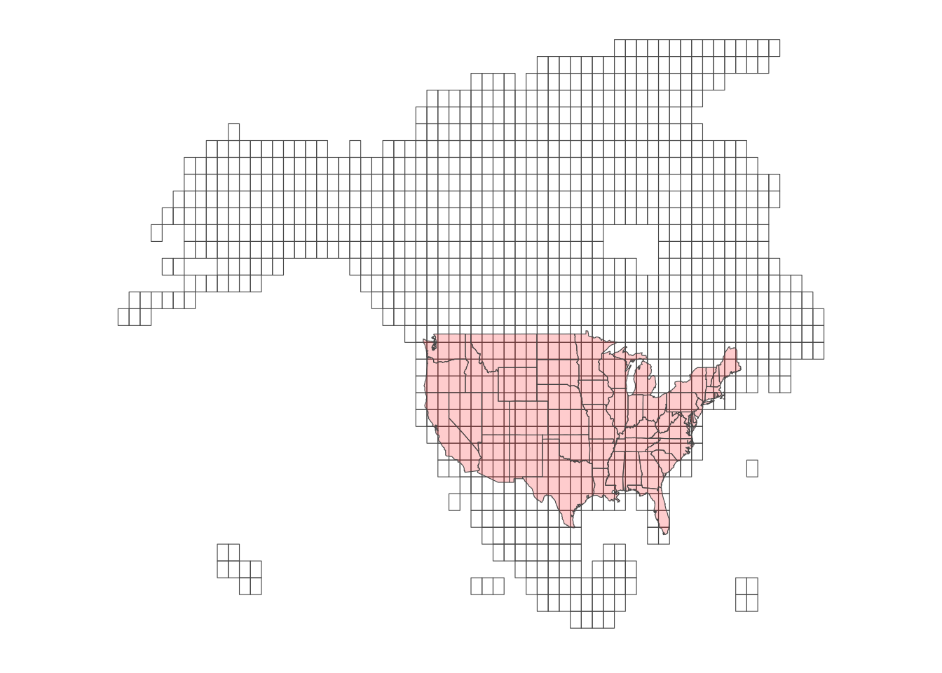
Figure 9.3: Daymet Tiles
Here is the list of weather variables:
- vapor pressure
- minimum and maximum temperature
- snow water equivalent
- solar radiation
- precipitation
- day length
So, Daymet provides information about more weather variables than PRISM, which helps to find some weather-dependent metrics, such as evapotranspiration.
The easiest way find Daymet values for your vector data depends on whether it is points or polygons data. For points data, daymetr::download_daymet() is the easiest because it will directly return weather values to the point of interest. Internally, it finds the cell in which the point is located, and then return the values of the cell for the specified length of period. daymetr::download_daymet() does all this for you. For polygons, we need to first download pertinent Daymet data for the region of interest first and then extract values for each of the polygons ourselves, which we learned in Chapter 5. Unfortunately, the netCDF data downloaded from daymetr::download_daymet_ncss() cannot be easily read by the raster package nor the stars package. On the contrary, FedData::get_daymet() download the the requested Daymet data and save it as a RasterBrick object, which can be easily turned into stars object using st_as_stars().
9.4.1 For points data
For points data, the easiest way to associate daily weather values to them is to use download_daymet(). download_daymet() can download daily weather data for a single point at a time by finding which cell of a tile the point is located within.
Here are key parameters for the function:
- lat: latitude
- lon: longitude
- start: start_year
- end: end_year
- internal:
TRUE(dafault) orFALSE
For example, the code below downloads daily weather data for a point (lat = \(36\), longitude = \(-100\)) starting from 2000 to 2002 and assigns the downloaded data to temp_daymet.
#--- download daymet data ---#
temp_daymet <- download_daymet(
  lat = 36,
  lon = -100,
  start = 2000,
  end = 2002
)

#--- structure ---#
str(temp_daymet)
List of 7
$ site : chr "Daymet"
$ tile : num 11380
$ latitude : num 36
$ longitude: num -100
$ altitude : num 746
$ tile : num 11380
$ data :'data.frame': 1095 obs. of 9 variables:
..$ year : int [1:1095] 2000 2000 2000 2000 2000 2000 2000 2000 2000 2000 ...
..$ yday : int [1:1095] 1 2 3 4 5 6 7 8 9 10 ...
..$ dayl..s. : num [1:1095] 34571 34606 34644 34685 34729 ...
..$ prcp..mm.day.: num [1:1095] 0 0 0 0 0 0 0 0 0 0 ...
..$ srad..W.m.2. : num [1:1095] 334 231 148 319 338 ...
..$ swe..kg.m.2. : num [1:1095] 18.2 15 13.6 13.6 13.6 ...
..$ tmax..deg.c. : num [1:1095] 20.9 13.88 4.49 9.18 13.37 ...
..$ tmin..deg.c. : num [1:1095] -2.73 1.69 -2.6 -10.16 -8.97 ...
..$ vp..Pa. : num [1:1095] 500 690 504 282 310 ...
- attr(*, "class")= chr "daymetr"As you can see, temp_daymet has bunch of site information other than the download Daymet data.
#--- get the data part ---#
temp_daymet_data <- temp_daymet$data

#--- take a look ---#
head(temp_daymet_data)
year yday dayl..s. prcp..mm.day. srad..W.m.2. swe..kg.m.2. tmax..deg.c.
1 2000 1 34571.11 0 334.34 18.23 20.90
2 2000 2 34606.19 0 231.20 15.00 13.88
3 2000 3 34644.13 0 148.29 13.57 4.49
4 2000 4 34684.93 0 319.13 13.57 9.18
5 2000 5 34728.55 0 337.67 13.57 13.37
6 2000 6 34774.96 0 275.72 13.11 9.98
tmin..deg.c. vp..Pa.
1 -2.73 499.56
2 1.69 689.87
3 -2.60 504.40
4 -10.16 282.35
5 -8.97 310.05
6 -4.89 424.78As you might have noticed, yday is not the date of each observation, but the day of the year. You can easily convert it into dates like this:
One dates are obtained, you can use the lubridate package to extract day, month, and year using day(), month(), and year(), respectively.
library(lubridate)

temp_daymet_data <- mutate(temp_daymet_data,
  day = day(date),
  month = month(date),
  #--- this is already there though ---#
  year = year(date)
)

#--- take a look ---#
dplyr::select(temp_daymet_data, year, month, day) %>% head()
year month day
1 2000 1 1
2 2000 1 2
3 2000 1 3
4 2000 1 4
5 2000 1 5
6 2000 1 6This helps you find group statistics like monthly precipitation.
# A tibble: 12 × 2
   month  prcp
   <dbl> <dbl>
 1     1 0.762
 2     2 1.20
 3     3 2.08
 4     4 1.24
 5     5 3.53
 6     6 3.45
 7     7 1.78
 8     8 1.19
 9     9 1.32
10    10 4.78
11    11 0.407
12    12 0.743
Downloading Daymet data for many points is just applying the same operations above to them using a loop. Let’s create random points within California and get their coordinates.
set.seed(389548)

random_points <-
  tigris::counties(state = "CA") %>%
  st_as_sf() %>%
  #--- 10 points ---#
  st_sample(10) %>%
  #--- get the coordinates ---#
  st_coordinates() %>%
  #--- as tibble (data.frame) ---#
  as_tibble() %>%
  #--- assign site id ---#
  mutate(site_id = 1:n())
To loop over the points, you can first write a function like this:
get_daymet <- function(i) {
  temp_lat <- random_points[i, ] %>% pull(Y)
  temp_lon <- random_points[i, ] %>% pull(X)
  temp_site <- random_points[i, ] %>% pull(site_id)

  temp_daymet <- download_daymet(
    lat = temp_lat,
    lon = temp_lon,
    start = 2000,
    end = 2002
  ) %>%
    #--- just get the data part ---#
    .$data %>%
    #--- convert to tibble (not strictly necessary) ---#
    as_tibble() %>%
    #--- assign site_id so you know which record is for which site_id ---#
    mutate(site_id = temp_site) %>%
    #--- get date from day of the year ---#
    mutate(date = as.Date(paste(year, yday, sep = "-"), "%Y-%j"))

  return(temp_daymet)
}
Here is what the function returns for the 1st row of random_points:
get_daymet(1)# A tibble: 1,095 × 11
year yday dayl..s. prcp..mm.day. srad..W.m.2. swe..kg.m.2. tmax..deg.c.
<int> <int> <dbl> <dbl> <dbl> <dbl> <dbl>
1 2000 1 34131. 0 246. 0 7.02
2 2000 2 34168. 0 251. 0 4.67
3 2000 3 34208. 0 247. 0 7.32
4 2000 4 34251 0 267. 0 10
5 2000 5 34297 0 240. 0 4.87
6 2000 6 34346. 0 274. 0 7.79
7 2000 7 34398. 0 262. 0 7.29
8 2000 8 34453. 0 291. 0 11.2
9 2000 9 34510. 0 268. 0 10.0
10 2000 10 34570. 0 277. 0 11.8
# ℹ 1,085 more rows
# ℹ 4 more variables: tmin..deg.c. <dbl>, vp..Pa. <dbl>, site_id <int>,
# date <date>You can now simply loop over the rows.
(
  daymet_all_points <- lapply(1:nrow(random_points), get_daymet) %>%
    #--- need to combine the list of data.frames into a single data.frame ---#
    bind_rows()
)
# A tibble: 10,950 × 11
year yday dayl..s. prcp..mm.day. srad..W.m.2. swe..kg.m.2. tmax..deg.c.
<dbl> <dbl> <dbl> <dbl> <dbl> <dbl> <dbl>
1 2000 1 33523. 0 230. 0 12
2 2000 2 33523. 0 240 0 11.5
3 2000 3 33523. 0 243. 0 13.5
4 2000 4 33523. 1 230. 0 13
5 2000 5 33523. 0 243. 0 14
6 2000 6 33523. 0 243. 0 13
7 2000 7 33523. 0 246. 0 14
8 2000 8 33869. 0 230. 0 13
9 2000 9 33869. 0 227. 0 12.5
10 2000 10 33869. 0 214. 0 14
# ℹ 10,940 more rows
# ℹ 4 more variables: tmin..deg.c. <dbl>, vp..Pa. <dbl>, site_id <int>,
# date <date>Or better yet, you can easily parallelize this process as follows (see Chapter A if you are not familiar with parallelization in R):
library(future.apply)
library(parallel)

#--- parallelization planning ---#
plan(multisession, workers = detectCores() - 1)

#--- parallelized lapply ---#
daymet_all_points <- future_lapply(1:nrow(random_points), get_daymet) %>%
  #--- need to combine the list of data.frames into a single data.frame ---#
  bind_rows()
9.4.2 For polygons data
Suppose you are interested in getting Daymet data for select counties in Michigan (Figure 9.4).
#--- entire MI ---#
MI_counties <- tigris::counties(state = "MI")

#--- select counties ---#
MI_counties_select <- filter(MI_counties, NAME %in% c("Luce", "Chippewa", "Mackinac"))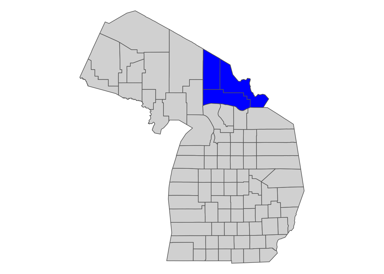
Figure 9.4: Select Michigan counties for which we download Daymet data
We can use FedData::get_daymet() to download Daymet data that covers the spatial extent of the polygons data. The downloaded dataset can be assigned to an R object as RasterBrick (you could alternatively write the downloaded data to a file). In order to let the function know the spatial extent for which it download Daymet data, we supply a SpatialPolygonsDataFrame object supported by the sp package. Since our main vector data handling package is sf we need to convert the sf object to a sp object.
The code below downloads prcp and tmax for the spatial extent of Michigan counties for 2000 and 2001:
(
  MI_daymet_select <- FedData::get_daymet(
    #--- supply the vector data in sp ---#
    template = as(MI_counties_select, "Spatial"),
    #--- label ---#
    label = "MI_counties_select",
    #--- variables to download ---#
    elements = c("prcp", "tmax"),
    #--- years ---#
    years = 2000:2001
  )
)
$prcp
class : RasterBrick
dimensions : 96, 156, 14976, 730 (nrow, ncol, ncell, nlayers)
resolution : 1000, 1000 (x, y)
extent : 1027250, 1183250, 455500, 551500 (xmin, xmax, ymin, ymax)
crs : +proj=lcc +lon_0=-100 +lat_0=42.5 +x_0=0 +y_0=0 +lat_1=25 +lat_2=60 +ellps=WGS84
source : memory
names : X2000.01.01, X2000.01.02, X2000.01.03, X2000.01.04, X2000.01.05, X2000.01.06, X2000.01.07, X2000.01.08, X2000.01.09, X2000.01.10, X2000.01.11, X2000.01.12, X2000.01.13, X2000.01.14, X2000.01.15, ...
min values : 0, 0, 0, 0, 0, 0, 0, 0, 0, 0, 0, 0, 0, 0, 0, ...
max values : 6, 26, 19, 17, 6, 9, 6, 1, 0, 13, 15, 6, 0, 4, 7, ...
$tmax
class : RasterBrick
dimensions : 96, 156, 14976, 730 (nrow, ncol, ncell, nlayers)
resolution : 1000, 1000 (x, y)
extent : 1027250, 1183250, 455500, 551500 (xmin, xmax, ymin, ymax)
crs : +proj=lcc +lon_0=-100 +lat_0=42.5 +x_0=0 +y_0=0 +lat_1=25 +lat_2=60 +ellps=WGS84
source : memory
names : X2000.01.01, X2000.01.02, X2000.01.03, X2000.01.04, X2000.01.05, X2000.01.06, X2000.01.07, X2000.01.08, X2000.01.09, X2000.01.10, X2000.01.11, X2000.01.12, X2000.01.13, X2000.01.14, X2000.01.15, ...
min values : 0.5, -4.5, -8.0, -8.5, -7.0, -2.5, -6.5, -1.5, 1.5, 2.0, -1.5, -8.5, -14.0, -9.5, -3.0, ...
max values : 3.0, 3.0, 0.5, -2.5, -2.5, 0.0, 0.5, 1.5, 4.0, 3.0, 3.5, 0.5, -6.5, -4.0, 0.0, ... As you can see, Daymet prcp and tmax data are stored separately as RasterBrick. Now that you have stars objects, you can extract values for your target polygons data using the methods described in Chapter 5.
If you use the stars package for raster data handling (see Chapter 7), you can convert them into stars object using st_as_stars().
#--- tmax as stars ---#
tmax_stars <- st_as_stars(MI_daymet_select$tmax)

#--- prcp as stars ---#
prcp_stars <- st_as_stars(MI_daymet_select$prcp)
Now, the third dimension (band) is not recognized as dates. We can use st_set_dimension() to change that (see Chapter 7.5). Before that, we first need to recover Date values from the “band” values as follows:
date_values <- tmax_stars %>%
  #--- get band values ---#
  st_get_dimension_values(., "band") %>%
  #--- remove X ---#
  gsub("X", "", .) %>%
  #--- convert to date ---#
  ymd(.)

#--- take a look ---#
head(date_values)
[1] "2000-01-01" "2000-01-02" "2000-01-03" "2000-01-04" "2000-01-05"
[6] "2000-01-06"
#--- tmax ---#
st_set_dimensions(tmax_stars, 3, values = date_values, names = "date")
stars object with 3 dimensions and 1 attribute
attribute(s), summary of first 1e+05 cells:
Min. 1st Qu. Median Mean 3rd Qu. Max. NA's
X2000.01.01 -8.5 -4 -2 -1.884266 0 3 198
dimension(s):
from to offset delta refsys
x 1 156 1027250 1000 +proj=lcc +lon_0=-100 +la...
y 1 96 551500 -1000 +proj=lcc +lon_0=-100 +la...
date 1 730 NA NA Date
values x/y
x NULL [x]
y NULL [y]
date 2000-01-01,...,2001-12-31
#--- prcp ---#
st_set_dimensions(prcp_stars, 3, values = date_values, names = "date")
stars object with 3 dimensions and 1 attribute
attribute(s), summary of first 1e+05 cells:
Min. 1st Qu. Median Mean 3rd Qu. Max. NA's
X2000.01.01 0 0 3 6.231649 12 26 198
dimension(s):
from to offset delta refsys
x 1 156 1027250 1000 +proj=lcc +lon_0=-100 +la...
y 1 96 551500 -1000 +proj=lcc +lon_0=-100 +la...
date 1 730 NA NA Date
values x/y
x NULL [x]
y NULL [y]
date 2000-01-01,...,2001-12-31 Notice that the date dimension has NA for delta. This is because Daymet removes observations for December 31 in leap years to make the time dimension 365 consistently across years. This means that there is a one-day gap between “2000-12-30” and “2000-01-01” as you can see below:
date_values[364:367][1] "2000-12-29" "2000-12-30" "2001-01-01" "2001-01-02"9.5 gridMET
gridMET is a dataset of daily meteorological data that covers the contiguous US since 1979. It spatial resolution is the same as PRISM data at 4-km by 4-km. Indeed gridMET is a product of combining PRISM and Land Data Assimilation System (https://ldas.gsfc.nasa.gov/nldas/NLDAS2forcing.php) (in particular NLDAS-2). It offer more variables than PRISM, including maximum temperature, minimum temperature, precipitation accumulation, downward surface shortwave radiation, wind-velocity, humidity (maximum and minimum relative humidity and specific humidity. It also offers derived products such as reference evapotranspiration (calculated based on Penman-Montieth equation).
You can use the downloadr::download() function to download gridMET data by variable-year. For example, to download precipitation data for 2018, you can run the following code:
downloader::download(
  url = "http://www.northwestknowledge.net/metdata/data/pr_2018.nc",
  destfile = "Data/pr_2018.nc",
  mode = "wb"
)
We set the url of the dataset of interest the url option, set the destination file name, and the mode to wb for a binary download.
All the gridMET datasets for direct download has “http://www.northwestknowledge.net/metdata/data/” at the beginning, followed by the file name (here, pr_2018.nc). The file names follow the convention of variable_abbreviation_year.nc. So, we can easily write a loop to get data for multiple variables over multiple years.
Here is the list of variable abbreviations:
- sph: (Near-Surface Specific Humidity)
- vpd: (Mean Vapor Pressure Deficit)
- pr: (Precipitation)
- rmin: (Minimum Near-Surface Relative Humidity)
- rmax: (Maximum Near-Surface Relative Humidity)
- srad: (Surface Downwelling Solar Radiation)
- tmmn: (Minimum Near-Surface Air Temperature)
- tmmx: (Maximum Near-Surface Air Temperature)
- vs: (Wind speed at 10 m)
- th: (Wind direction at 10 m)
- pdsi: (Palmer Drought Severity Index)
- pet: (Reference grass evaportranspiration)
- etr: (Reference alfalfa evaportranspiration)
- erc: (model-G)
- bi: (model-G)
- fm100: (100-hour dead fuel moisture)
- fm1000: (1000-hour dead fuel moisture)
As another example, if you are interested in downloading the wind speed data for 2020, then you can use the following code.
downloader::download(
  url = "http://www.northwestknowledge.net/metdata/data/vs_2020.nc",
  destfile = "Data/vs_2020.nc",
  mode = "wb"
)
9.5.1 Practical Examples
Suppose your final goal is to get average daily precipitation (pr) and reference grass evapotranspiration (pet) from 2015 through 2020 for each of the counties in California.
First get county boundaries for California:
Before writing a loop, let’s work on a single case (pet for 2015). First, we download and read the data.
#--- download data ---#
downloader::download(
  url = "http://www.northwestknowledge.net/metdata/data/pet_2015.nc",
  destfile = "Data/pet_2015.nc",
  mode = "wb"
)

#--- read the raster data ---#
(
  pet_2015 <- rast("Data/pet_2015.nc")
)
class : SpatRaster
dimensions : 585, 1386, 365 (nrow, ncol, nlyr)
resolution : 0.04166667, 0.04166667 (x, y)
extent : -124.7875, -67.0375, 25.04583, 49.42083 (xmin, xmax, ymin, ymax)
coord. ref. : lon/lat WGS 84 (EPSG:4326)
source : pet_2015.nc
varname : potential_evapotranspiration (pet)
names : poten~42003, poten~42004, poten~42005, poten~42006, poten~42007, poten~42008, ...
unit : mm, mm, mm, mm, mm, mm, ... As you can see, it is a multi-layer raster object where each layer represents a single day in 2015. Here is a quick visualization of the first layer.
plot(pet_2015[[1]])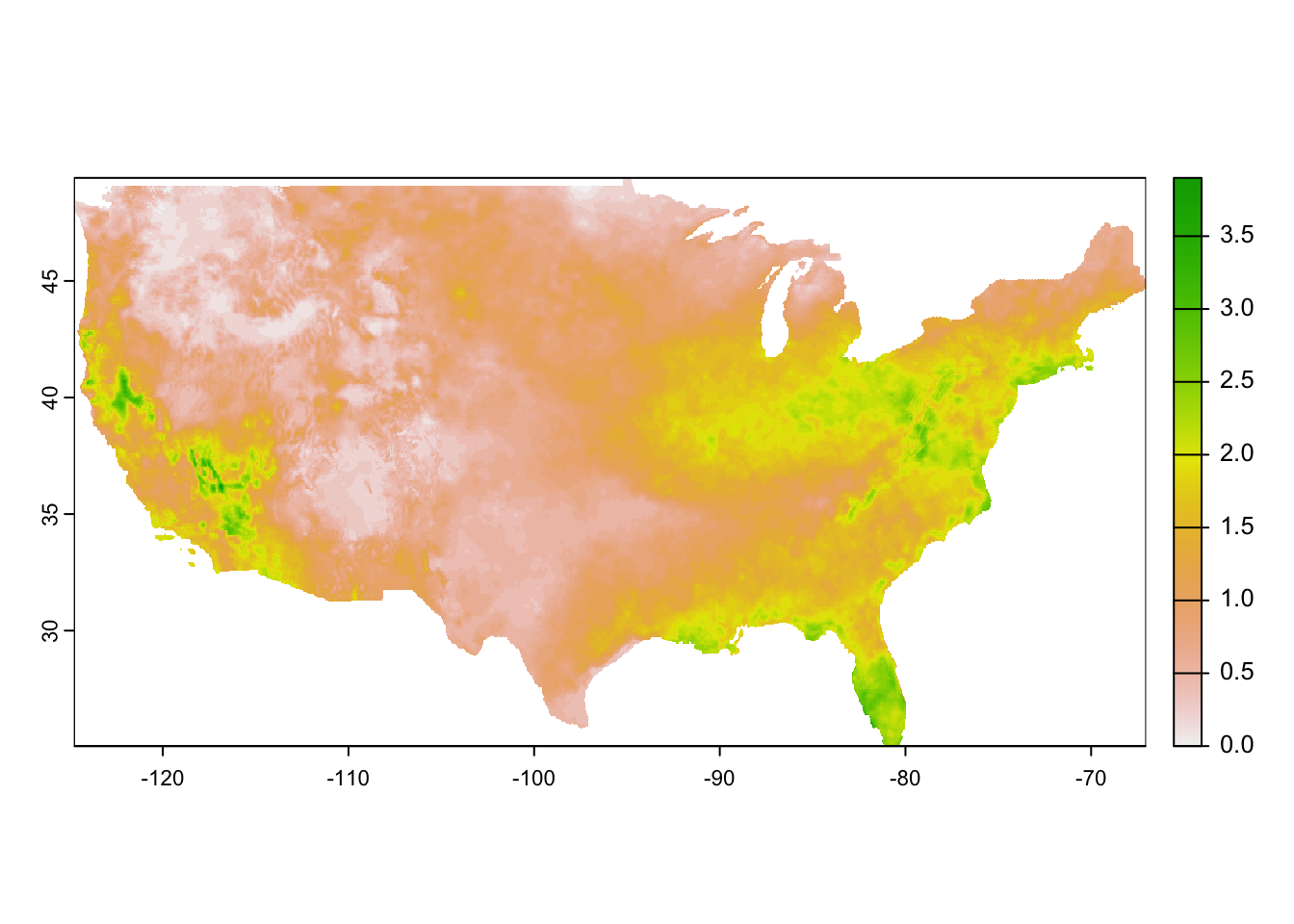
Now, we can use exactexactr::exact_extract() to assign cell values to each county and transform it to a more convenient form:
pet_county <-
  #--- extract data for each county ---#
  exact_extract(pet_2015, CA_counties, progress = FALSE) %>%
  #--- list of data.frames into data.table ---#
  rbindlist(idcol = "rowid")

#--- check the dimension of the output ---#
dim(pet_county)
[1] 28203 367As you can see the data has 367 columns: 365 (days) + 1 (rowid) + 1 (coverage fraction). Let’s take a look at the name of the first six variables.
[1] "rowid"
[2] "potential_evapotranspiration_day=42003"
[3] "potential_evapotranspiration_day=42004"
[4] "potential_evapotranspiration_day=42005"
[5] "potential_evapotranspiration_day=42006"
[6] "potential_evapotranspiration_day=42007"
The 5-digit number at the end of the name of the variables for evapotranspiration represents days since Jan 1st, 1900. This can be confirmed using ncdf4:nc_open() (see the middle of the output below under day of 4 dimensions):
ncdf4::nc_open("Data/pet_2015.nc")File Data/pet_2015.nc (NC_FORMAT_NETCDF4):
1 variables (excluding dimension variables):
unsigned short potential_evapotranspiration[lon,lat,day] (Chunking: [231,98,61]) (Compression: level 9)
_FillValue: 32767
units: mm
description: Daily reference evapotranspiration (short grass)
long_name: pet
standard_name: pet
missing_value: 32767
dimensions: lon lat time
grid_mapping: crs
coordinate_system: WGS84,EPSG:4326
scale_factor: 0.1
add_offset: 0
coordinates: lon lat
_Unsigned: true
4 dimensions:
lon Size:1386
units: degrees_east
description: longitude
long_name: longitude
standard_name: longitude
axis: X
lat Size:585
units: degrees_north
description: latitude
long_name: latitude
standard_name: latitude
axis: Y
day Size:365
description: days since 1900-01-01
units: days since 1900-01-01 00:00:00
long_name: time
standard_name: time
calendar: gregorian
crs Size:1
grid_mapping_name: latitude_longitude
longitude_of_prime_meridian: 0
semi_major_axis: 6378137
long_name: WGS 84
inverse_flattening: 298.257223563
GeoTransform: -124.7666666333333 0.041666666666666 0 49.400000000000000 -0.041666666666666
spatial_ref: GEOGCS["WGS 84",DATUM["WGS_1984",SPHEROID["WGS 84",6378137,298.257223563,AUTHORITY["EPSG","7030"]],AUTHORITY["EPSG","6326"]],PRIMEM["Greenwich",0,AUTHORITY["EPSG","8901"]],UNIT["degree",0.0174532925199433,AUTHORITY["EPSG","9122"]],AUTHORITY["EPSG","4326"]]
19 global attributes:
geospatial_bounds_crs: EPSG:4326
Conventions: CF-1.6
geospatial_bounds: POLYGON((-124.7666666333333 49.400000000000000, -124.7666666333333 25.066666666666666, -67.058333300000015 25.066666666666666, -67.058333300000015 49.400000000000000, -124.7666666333333 49.400000000000000))
geospatial_lat_min: 25.066666666666666
geospatial_lat_max: 49.40000000000000
geospatial_lon_min: -124.7666666333333
geospatial_lon_max: -67.058333300000015
geospatial_lon_resolution: 0.041666666666666
geospatial_lat_resolution: 0.041666666666666
geospatial_lat_units: decimal_degrees north
geospatial_lon_units: decimal_degrees east
coordinate_system: EPSG:4326
author: John Abatzoglou - University of Idaho, jabatzoglou@uidaho.edu
date: 04 July 2019
note1: The projection information for this file is: GCS WGS 1984.
note2: Citation: Abatzoglou, J.T., 2013, Development of gridded surface meteorological data for ecological applications and modeling, International Journal of Climatology, DOI: 10.1002/joc.3413
note3: Data in slices after last_permanent_slice (1-based) are considered provisional and subject to change with subsequent updates
note4: Data in slices after last_provisional_slice (1-based) are considered early and subject to change with subsequent updates
note5: Days correspond approximately to calendar days ending at midnight, Mountain Standard Time (7 UTC the next calendar day)This is universally true for all the gridMET data. We can use this information to recover date. First, let’s transform the data from a wide format to a long format for easier operations:
pet_county <-
  #--- wide to long ---#
  melt(pet_county, id.var = c("rowid", "coverage_fraction")) %>%
  #--- remove observations with NA values ---#
  .[!is.na(value), ]

#--- take a look ---#
pet_county
rowid coverage_fraction variable value
<int> <num> <fctr> <num>
1: 1 0.004266545 potential_evapotranspiration_day=42003 2.3
2: 1 0.254054248 potential_evapotranspiration_day=42003 2.2
3: 1 0.175513789 potential_evapotranspiration_day=42003 2.0
4: 1 0.442011684 potential_evapotranspiration_day=42003 2.1
5: 1 1.000000000 potential_evapotranspiration_day=42003 2.2
---
10116701: 58 0.538234591 potential_evapotranspiration_day=42367 2.1
10116702: 58 0.197555855 potential_evapotranspiration_day=42367 2.7
10116703: 58 0.224901110 potential_evapotranspiration_day=42367 2.2
10116704: 58 0.554238617 potential_evapotranspiration_day=42367 2.2
10116705: 58 0.272462875 potential_evapotranspiration_day=42367 2.1We now use str_sub() to get 5-digit numbers from variable, which represents days since Jan 1st, 1900. We can then recover dates using the lubridate package.
pet_county[, variable := str_sub(variable, -5, -1) %>% as.numeric()] %>%
  #--- recover dates ---#
  .[, date := variable + lubridate::ymd("1900-01-01")]

#--- take a look ---#
pet_county
rowid coverage_fraction variable value date
<int> <num> <num> <num> <Date>
1: 1 0.004266545 42003 2.3 2015-01-01
2: 1 0.254054248 42003 2.2 2015-01-01
3: 1 0.175513789 42003 2.0 2015-01-01
4: 1 0.442011684 42003 2.1 2015-01-01
5: 1 1.000000000 42003 2.2 2015-01-01
---
10116701: 58 0.538234591 42367 2.1 2015-12-31
10116702: 58 0.197555855 42367 2.7 2015-12-31
10116703: 58 0.224901110 42367 2.2 2015-12-31
10116704: 58 0.554238617 42367 2.2 2015-12-31
10116705: 58 0.272462875 42367 2.1 2015-12-31Finally, let’s calculate the coverage-weighted average of pet by county-date.
pet_county_avg <-
  pet_county[,
    .(value = sum(value * coverage_fraction) / sum(coverage_fraction)),
    by = .(rowid, date)
  ] %>%
  setnames("value", "pet")
Since rowid value of n corresponds to the n th row in CA_counties, it is easy to merge pet_county_avg with CA_counties (alternatively, you can use cbind()).
CA_pet <- CA_counties %>%
  mutate(rowid = seq_len(nrow(.))) %>%
  left_join(pet_county_avg, ., by = "rowid")
Now that we know how to process a single gridMET dataset, we are ready to write a function that goes through the same for a choice of gridMET dataset and then write a loop to achieve our goal. Here is the function:
get_grid_MET <- function(var_name, year) {
  #--- for testing ---#
  # var_name <- "pet"
  # year <- 2020

  target_url <-
    paste0(
      "http://www.northwestknowledge.net/metdata/data/",
      var_name, "_", year,
      ".nc"
    )

  file_name <-
    paste0(
      "Data/",
      var_name, "_", year,
      ".nc"
    )

  downloader::download(
    url = target_url,
    destfile = file_name,
    mode = "wb"
  )

  #--- read the raster data ---#
  temp_rast <- rast(file_name)

  temp_data <-
    #--- extract data for each county ---#
    exact_extract(temp_rast, CA_counties) %>%
    #--- list of data.frames into data.table ---#
    rbindlist(idcol = "rowid") %>%
    #--- wide to long ---#
    melt(id.var = c("rowid", "coverage_fraction")) %>%
    #--- remove observations with NA values ---#
    .[!is.na(value), ] %>%
    #--- get only the numeric part ---#
    .[, variable := str_sub(variable, -5, -1) %>% as.numeric()] %>%
    #--- recover dates ---#
    .[, date := variable + ymd("1900-01-01")] %>%
    #--- find daily coverage-weight average by county ---#
    .[,
      .(value = sum(value * coverage_fraction) / sum(coverage_fraction)),
      by = .(rowid, date)
    ] %>%
    .[, var := var_name]

  return(temp_data)
}
Let’s now loop over the variables and years of interest. We first set up a dataset of variable-year combinations for which we loop over.
#--- create a dataset of parameters to be looped over---#
(
  par_data <-
    expand.grid(
      var_name = c("pr", "pet"),
      year = 2015:2020
    ) %>%
    data.table() %>%
    .[, var_name := as.character(var_name)]
)
We now loop over the rows of par_data in parallel:
#--- parallel processing ---#
library(future.apply)
plan(multisession, workers = 12)

(
  all_data <-
    future_lapply(
      seq_len(nrow(par_data)),
      function(x) get_grid_MET(par_data[x, var_name], par_data[x, year])
    ) %>%
    rbindlist() %>%
    dcast(rowid + date ~ var, value.var = "value")
)