2.5 Quick and interactive view of an sf object

2.5.1 Quick view

The easiest way to visualize an sf object is to use plot():

plot(nc)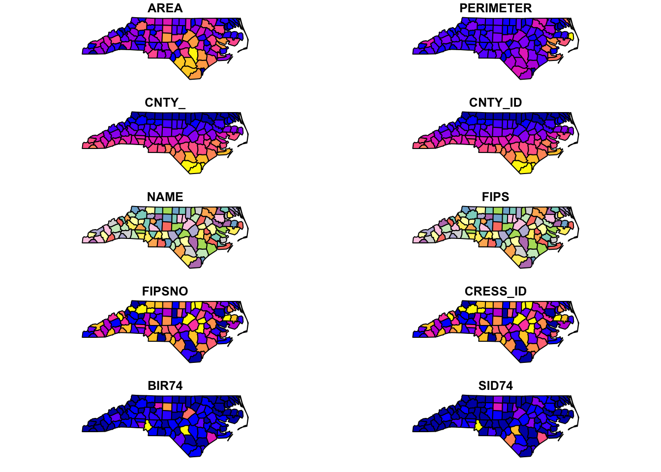

Figure 2.2: Quick Visualization of an sf object

As you can see, plot() create a map for each variable where the spatial units are color-differentiated based on the values of the variable. For creating more elaborate maps that are of publication-quality, see Chapter 8.

2.5.2 Interactive view

Sometimes it is useful to be able to tell where certain spatial objects are and what values are associated with them on a map. The tmap_leaflet() function from the tmap package can create an interactive map where you can point to a spatial object and the associated information is revealed on the map. Let’s use the North Carolina county map as an example here:

Figure 2.3: Interactive map of North Carolina counties

As you can see, if you put your cursor on a polygon (county) and click on it, then its information pops up.

---

Alternatively, you could use the tmap package to create interactive maps. You can first create a static map following a syntax like this:

#--- NOT RUN (for polygons) ---#
tm_shape(sf) +
  tm_polygons()

#--- NOT RUN (for points) ---#
tm_shape(sf) +
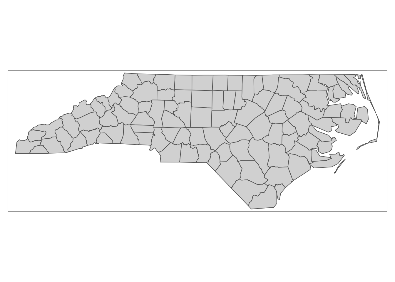
  tm_symbols()

This creates a static map of nc where county boundaries are drawn:

(
  tm_nc_polygons <- tm_shape(nc) + tm_polygons()
)

Then, you can apply tmap_leaflet() to the static map to have an interactive view of the map:

tmap_leaflet(tm_nc_polygons)

You could also change the view mode of tmap objects to the view mode using tmap_mode("view") and then simply evaluate tm_nc_polygons.

#--- change to the "view" mode ---#
tmap_mode("view")

#--- now you have an interactive biew ---#
tm_nc_polygons

Note that once you change the view mode to “view,” then the evaluation of all tmap objects become interactive. I prefer the first option, as I need to revert the view mode back to “plot” by tmap_mode("plot") if I don’t want interactive views.