3.1 Topological relations
Before we learn spatial subsetting and joining, we first look at topological relations. Topological relations refer to the way multiple spatial objects are spatially related to one another. You can identify various types of spatial relations using the sf package. Our main focus is on the intersections of spatial objects, which can be found using st_intersects()56. We also briefly cover st_is_within_distance(). If you are interested in other topological relations, run ?geos_binary_pred.
We first create sf objects we are going to use for illustrations.
POINTS
#--- create points ---#
point_1 <- st_point(c(2, 2))
point_2 <- st_point(c(1, 1))
point_3 <- st_point(c(1, 3))

#--- combine the points to make a single  sf of points ---#
(
points <- list(point_1, point_2, point_3) %>%
  st_sfc() %>%
  st_as_sf() %>%
  mutate(point_name = c("point 1", "point 2", "point 3"))
)
Simple feature collection with 3 features and 1 field
Geometry type: POINT
Dimension: XY
Bounding box: xmin: 1 ymin: 1 xmax: 2 ymax: 3
CRS: NA
x point_name
1 POINT (2 2) point 1
2 POINT (1 1) point 2
3 POINT (1 3) point 3LINES
#--- create points ---#
line_1 <- st_linestring(rbind(c(0, 0), c(2.5, 0.5)))
line_2 <- st_linestring(rbind(c(1.5, 0.5), c(2.5, 2)))

#--- combine the points to make a single  sf of points ---#
(
lines <- list(line_1, line_2) %>%
  st_sfc() %>%
  st_as_sf() %>%
  mutate(line_name = c("line 1", "line 2"))
)
Simple feature collection with 2 features and 1 field
Geometry type: LINESTRING
Dimension: XY
Bounding box: xmin: 0 ymin: 0 xmax: 2.5 ymax: 2
CRS: NA
x line_name
1 LINESTRING (0 0, 2.5 0.5) line 1
2 LINESTRING (1.5 0.5, 2.5 2) line 2POLYGONS
#--- create polygons ---#
polygon_1 <- st_polygon(list(
  rbind(c(0, 0), c(2, 0), c(2, 2), c(0, 2), c(0, 0))
))

polygon_2 <- st_polygon(list(
  rbind(c(0.5, 1.5), c(0.5, 3.5), c(2.5, 3.5), c(2.5, 1.5), c(0.5, 1.5))
))

polygon_3 <- st_polygon(list(
  rbind(c(0.5, 2.5), c(0.5, 3.2), c(2.3, 3.2), c(2, 2), c(0.5, 2.5))
))

#--- combine the polygons to make an sf of polygons ---#
(
polygons <- list(polygon_1, polygon_2, polygon_3) %>%
  st_sfc() %>%
  st_as_sf() %>%
  mutate(polygon_name = c("polygon 1", "polygon 2", "polygon 3"))
)
Simple feature collection with 3 features and 1 field
Geometry type: POLYGON
Dimension: XY
Bounding box: xmin: 0 ymin: 0 xmax: 2.5 ymax: 3.5
CRS: NA
x polygon_name
1 POLYGON ((0 0, 2 0, 2 2, 0 ... polygon 1
2 POLYGON ((0.5 1.5, 0.5 3.5,... polygon 2
3 POLYGON ((0.5 2.5, 0.5 3.2,... polygon 3Figure 3.1 shows how they look:
ggplot() +
  geom_sf(data = polygons, aes(fill = polygon_name), alpha = 0.3) +
  scale_fill_discrete(name = "Polygons") +
  geom_sf(data = lines, aes(color = line_name)) +
  scale_color_discrete(name = "Lines") +
  geom_sf(data = points, aes(shape = point_name), size = 3) +
scale_shape_discrete(name = "Points") 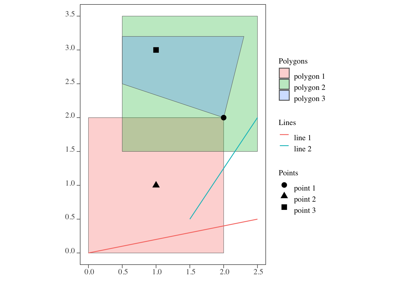
Figure 3.1: Visualization of the points, lines, and polygons
3.1.1 st_intersects()
This function identifies which sfg object in an sf (or sfc) intersects with sfg object(s) in another sf. For example, you can use the function to identify which well is located within which county. st_intersects() is the most commonly used topological relation. It is important to understand what it does as it is the default topological relation used when performing spatial subsetting and joining, which we will cover later.
points and polygons
st_intersects(points, polygons)Sparse geometry binary predicate list of length 3, where the predicate
was `intersects'
1: 1, 2, 3
2: 1
3: 2, 3As you can see, the output is a list of which polygon(s) each of the points intersect with. The numbers 1, 2, and 3 in the first row mean that 1st (polygon 1), 2nd (polygon 2), and 3rd (polygon 3) objects of the polygons intersect with the first point (point 1) of the points object. The fact that point 1 is considered to be intersecting with polygon 2 means that the area inside the border is considered a part of the polygon (of course).
If you would like the results of st_intersects() in a matrix form with boolean values filling the matrix, you can add sparse = FALSE option.
st_intersects(points, polygons, sparse = FALSE) [,1] [,2] [,3]
[1,] TRUE TRUE TRUE
[2,] TRUE FALSE FALSE
[3,] FALSE TRUE TRUElines and polygons
st_intersects(lines, polygons)Sparse geometry binary predicate list of length 2, where the predicate
was `intersects'
1: 1
2: 1, 2The output is a list of which polygon(s) each of the lines intersect with.
polygons and polygons
For polygons vs polygons interaction, st_intersects() identifies any polygons that either touches (even at a point like polygons 1 and 3) or share some area.
st_intersects(polygons, polygons)Sparse geometry binary predicate list of length 3, where the predicate
was `intersects'
1: 1, 2, 3
2: 1, 2, 3
3: 1, 2, 33.1.2 st_is_within_distance()
This function identifies whether two spatial objects are within the distance you specify as the name suggests57.
Let’s first create two sets of points.
set.seed(38424738)

points_set_1 <- lapply(1:5, function(x) st_point(runif(2))) %>%
  st_sfc() %>% st_as_sf() %>%
  mutate(id = 1:nrow(.))

points_set_2 <- lapply(1:5, function(x) st_point(runif(2))) %>%
  st_sfc() %>% st_as_sf() %>%
  mutate(id = 1:nrow(.))
Here is how they are spatially distributed (Figure 3.2). Instead of circles of points, their corresponding id (or equivalently row number here) values are displayed.
ggplot() +
  geom_sf_text(data = points_set_1, aes(label = id), color = "red") +
geom_sf_text(data = points_set_2, aes(label = id), color = "blue") 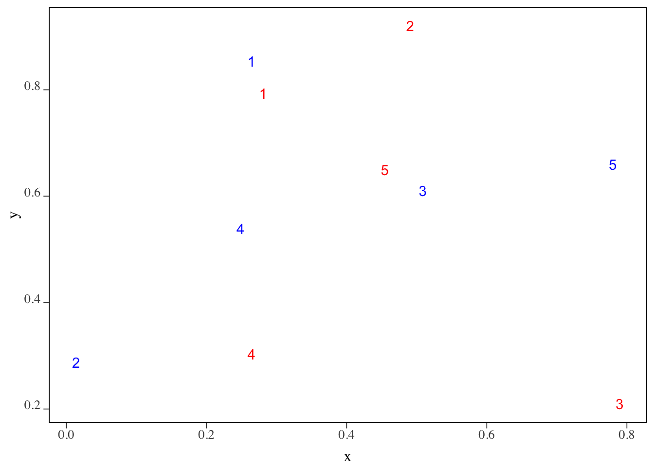
Figure 3.2: The locations of the set of points
We want to know which of the blue points (points_set_2) are located within 0.2 from each of the red points (points_set_1). The following figure (Figure 3.3) gives us the answer visually.
#--- create 0.2 buffers around points in points_set_1 ---#
buffer_1 <- st_buffer(points_set_1, dist = 0.2)

ggplot() +
  geom_sf(data = buffer_1, color = "red", fill = NA) +
  geom_sf_text(data = points_set_1, aes(label = id), color = "red") +
geom_sf_text(data = points_set_2, aes(label = id), color = "blue") 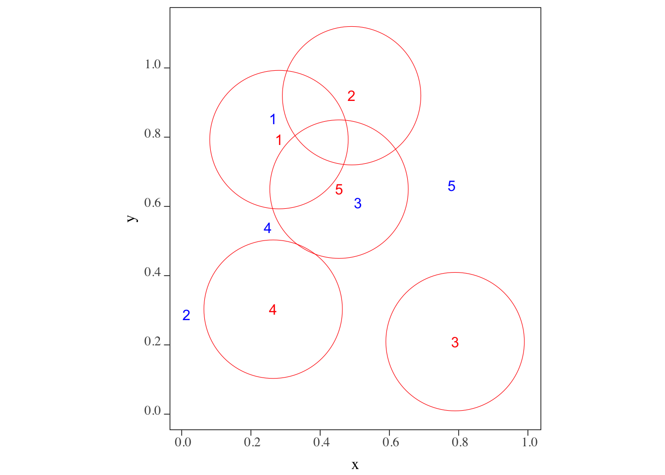
Figure 3.3: The blue points within 0.2 radius of the red points
Confirm your visual inspection results with the outcome of the following code using st_is_within_distance() function.
st_is_within_distance(points_set_1, points_set_2, dist = 0.2)Sparse geometry binary predicate list of length 5, where the predicate
was `is_within_distance'
1: 1
2: (empty)
3: (empty)
4: (empty)
5: 3