1.3 Demonstration 3: Land Use and Weather
1.3.1 Project Overview
Objective
- Understand the impact of past precipitation on crop choice in Iowa (IA).
Datasets
- IA county boundary
- Regular grids over IA, created using
sf::st_make_grid() - PRISM daily precipitation data downloaded using
prismpackage - Land use data from the Cropland Data Layer (CDL) for IA in 2015, downloaded using
cdlToolspackage
Econometric Model
The econometric model we would like to estimate is:
\[ CS_i = \alpha + \beta_1 PrN_{i} + \beta_2 PrC_{i} + v_i \] where \(CS_i\) is the area share of corn divided by that of soy in 2015 for grid \(i\) (we will generate regularly-sized grids in the Demo section), \(PrN_i\) is the total precipitation observed in April through May and September in 2014, \(PrC_i\) is the total precipitation observed in June through August in 2014, and \(v_i\) is the error term. To run the econometric model, we need to find crop share and weather variables observed at the grids. We first tackle the crop share variable, and then the precipitation variable.
GIS tasks
- download Cropland Data Layer (CDL) data by USDA NASS
- use
cdlTools::getCDL()
- use
- download PRISM weather data
- use
prism::get_prism_dailys()
- use
- crop PRISM data to the geographic extent of IA
- use
raster::crop()
- use
- create regular grids within IA, which become the observation units of the econometric analysis
- use
sf::st_make_grid()
- use
- remove grids that share small area with IA
- use
sf::st_intersection()andsf::st_area
- use
- assign crop share and weather data to each of the generated IA grids (parallelized)
- use
exactextractr::exact_extract()andfuture.apply::future_lapply()
- use
- create maps
- use the
tmappackage
- use the
Preparation for replication
- Run the following code to install or load (if already installed) the
pacmanpackage, and then install or load (if already installed) the listed package inside thepacman::p_load()function.
if (!require("pacman")) install.packages("pacman")
pacman::p_load(
  sf, # vector data operations
  raster, # raster data operations
  exactextractr, # fast raster data extraction for polygons
  maps, # to get county boundary data
  data.table, # data wrangling
  dplyr, # data wrangling
  lubridate, # Date object handling
  tmap, # for map creation
  stargazer, # regression table generation
  future.apply, # parallel computation
  cdlTools, # download CDL data
  rgdal, # required for cdlTools
  prism, # download PRISM data
  stringr # string manipulation
)
1.3.2 Project Demonstration
The geographic focus of this project is Iowas. Let’s get Iowa state border (see Figure 1.8 for its map).
#--- IA state boundary ---#
IA_boundary <- st_as_sf(maps::map("state", "iowa", plot = FALSE, fill = TRUE)) 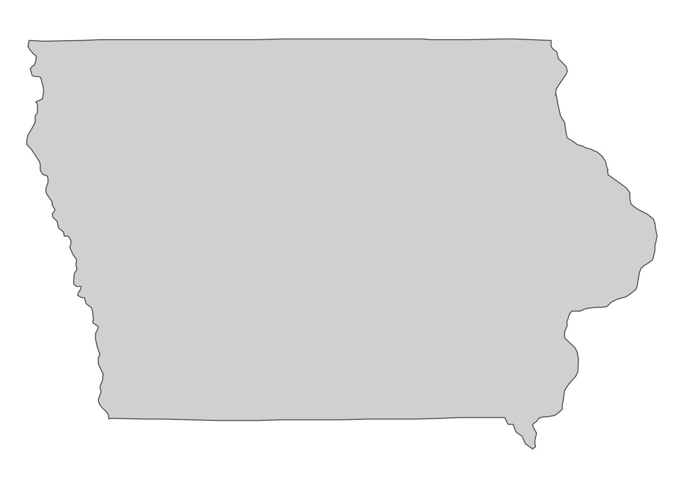
Figure 1.8: Iowa state boundary
The unit of analysis is artificial grids that we create over Iowa. The grids are regularly-sized rectangles except around the edge of the Iowa state border17. So, let’s create grids and remove those that do not overlap much with Iowa.
#--- create regular grids (40 cells by 40 columns) over IA ---#
IA_grids <- IA_boundary %>%
  #--- create grids ---#
  st_make_grid(, n = c(40, 40)) %>%
  #--- convert to sf ---#
  st_as_sf() %>%
  #--- find the intersections of IA grids and IA polygon ---#
  st_intersection(., IA_boundary) %>%
  #--- calculate the area of each grid ---#
  mutate(
    area = as.numeric(st_area(.)),
    area_ratio = area/max(area)
  ) %>%
  #--- keep only if the intersected area is large enough ---#
  filter(area_ratio > 0.8) %>%
  #--- assign grid id for future merge ---#
  mutate(grid_id = 1:nrow(.))
Here is what the generated grids look like (Figure 1.9):
#--- plot the grids over the IA state border ---#
tm_shape(IA_boundary) +
  tm_polygons(col = "green") +
tm_shape(IA_grids) +
  tm_polygons(alpha = 0) +
  tm_layout(frame = FALSE)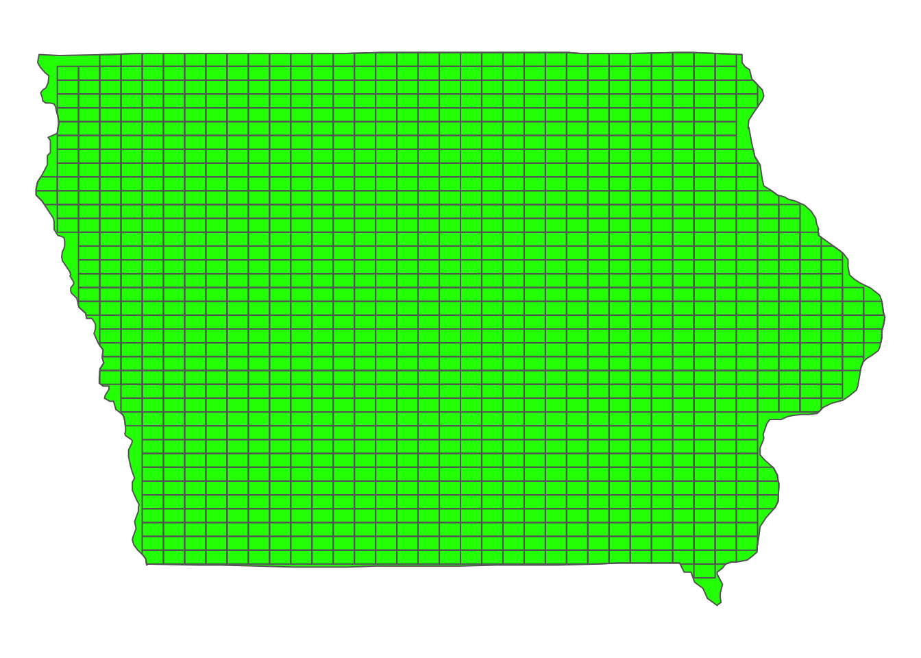
Figure 1.9: Map of regular grids generated over IA
Let’s work on crop share data. You can download CDL data using the getCDL() function from the cdlTools package.
The cells (30 meter by 30 meter) of the imported raster layer take a value ranging from 0 to 255. Corn and soybean are represented by 1 and 5, respectively (Figure 1.10).
Figure 1.10 shows the map of one of the IA grids and the CDL cells it overlaps with.
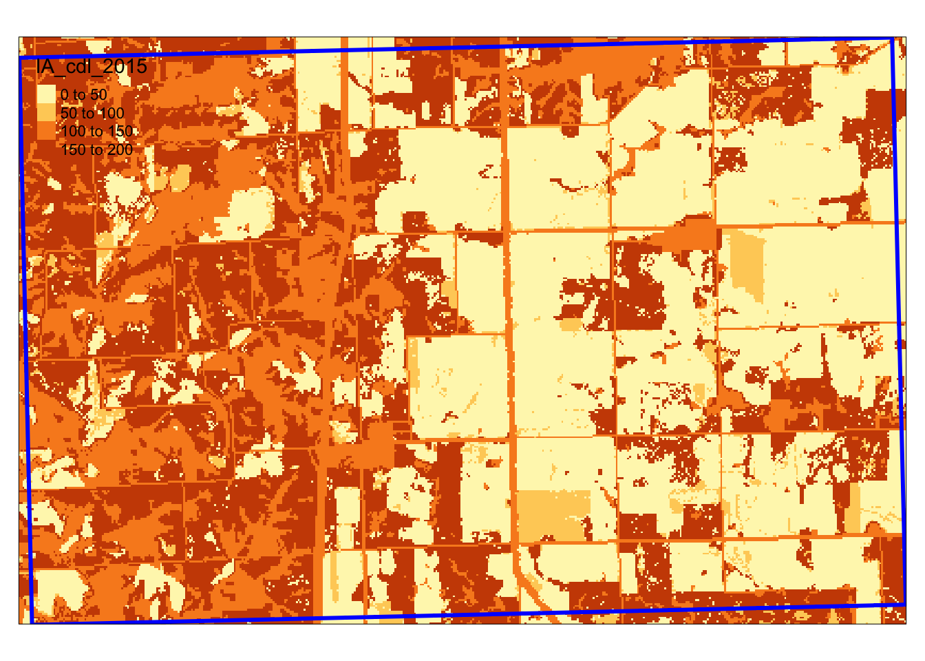
Figure 1.10: Spatial overlap of a IA grid and CDL layer
We would like to extract all the cell values within the blue border.
We use exactextractr::exact_extract() to identify which cells of the CDL raster layer fall within each of the IA grids and extract land use type values. We then find the share of corn and soybean for each of the grids.
#--- reproject grids to the CRS of the CDL data ---#
IA_grids_rp_cdl <- st_transform(IA_grids, projection(IA_cdl_2015))

#--- extract crop type values and find frequencies ---#
cdl_extracted <- exact_extract(IA_cdl_2015, IA_grids_rp_cdl) %>%
  lapply(., function (x) data.table(x)[,.N, by = value]) %>%
  #--- combine the list of data.tables into one data.table ---#
  rbindlist(idcol = TRUE) %>%
  #--- find the share of each land use type ---#
  .[, share := N/sum(N), by = .id] %>%
  .[, N := NULL] %>%
  #--- keep only the share of corn and soy ---#
  .[value %in% c(1, 5), ]
We then find the corn to soy ratio for each of the IA grids.
#--- find corn/soy ratio ---#
corn_soy <- cdl_extracted %>%
  #--- long to wide ---#
  dcast(.id ~ value, value.var = "share") %>%
  #--- change variable names ---#
  setnames(c(".id", "1", "5"), c("grid_id", "corn_share", "soy_share")) %>%
  #--- corn share divided by soy share ---#
  .[, c_s_ratio := corn_share / soy_share]
We are still missing daily precipitation data at the moment. We have decided to use daily weather data from PRISM. Daily PRISM data is a raster data with the cell size of 4 km by 4 km. Figure 1.11 presents precipitation data downloaded for April 1, 2010. It covers the entire contiguous U.S.
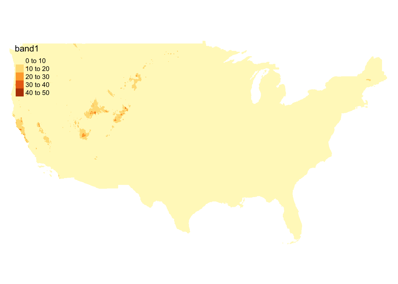
Figure 1.11: Map of PRISM raster data layer
Let’s now download PRISM data18. This can be done using the get_prism_dailys() function from the prism package.19
options(prism.path = "./Data/PRISM")

get_prism_dailys(
  type = "ppt",
  minDate = "2014-04-01",
  maxDate = "2014-09-30",
  keepZip = FALSE
)
When we use get_prism_dailys() to download data20, it creates one folder for each day. So, I have about 180 folders inside the folder I designated as the download destination above with the options() function.
We now try to extract precipitation value by day for each of the IA grids by geographically overlaying IA grids onto the PRISM data layer and identify which PRISM cells each of the IA grid encompass. Figure 1.12 shows how the first IA grid overlaps with the PRISM cells21.
#--- read a PRISM dataset ---#
prism_whole <- raster("./Data/PRISM/PRISM_ppt_stable_4kmD2_20140401_bil/PRISM_ppt_stable_4kmD2_20140401_bil.bil")

#--- align the CRS ---#
IA_grids_rp_prism <- st_transform(IA_grids, projection(prism_whole))

#--- crop the PRISM data for the 1st IA grid ---#
PRISM_1 <- crop(prism_whole, st_buffer(IA_grids_rp_prism[1, ], dist = 0.05))

#--- map them ---#
tm_shape(PRISM_1) +
  tm_raster() +
tm_shape(IA_grids_rp_prism[1, ]) +
  tm_polygons(alpha = 0) +
  tm_layout(frame = NA)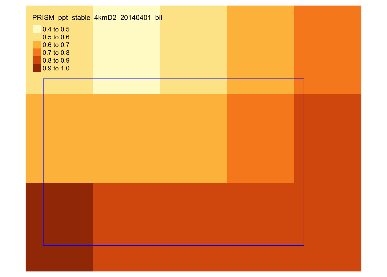
Figure 1.12: Spatial overlap of an IA grid over PRISM cells
As you can see, some PRISM grids are fully inside the analysis grid, while others are partially inside it. So, when assigning precipitation values to grids, we will use the coverage-weighted mean of precipitations22.
Unlike the CDL layer, we have 183 raster layers to process. Fortunately, we can process many raster files at the same time very quickly by first “stacking” many raster files first and then applying the exact_extract() function. Using future_lapply(), we let \(6\) cores take care of this task with each processing 31 files, except one of them handling only 28 files.23
We first get all the paths to the PRISM files.
#--- get all the dates ---#
dates_ls <- seq(as.Date("2014-04-01"), as.Date("2014-09-30"), "days")

#--- remove hyphen ---#
dates_ls_no_hyphen <- str_remove_all(dates_ls, "-")

#--- get all the prism file names ---#
folder_name <- paste0("PRISM_ppt_stable_4kmD2_", dates_ls_no_hyphen, "_bil")
file_name <- paste0("PRISM_ppt_stable_4kmD2_", dates_ls_no_hyphen, "_bil.bil")
file_paths <- paste0("./Data/PRISM/", folder_name, "/", file_name)

#--- take a look ---#
head(file_paths)
[1] "./Data/PRISM/PRISM_ppt_stable_4kmD2_20140401_bil/PRISM_ppt_stable_4kmD2_20140401_bil.bil"
[2] "./Data/PRISM/PRISM_ppt_stable_4kmD2_20140402_bil/PRISM_ppt_stable_4kmD2_20140402_bil.bil"
[3] "./Data/PRISM/PRISM_ppt_stable_4kmD2_20140403_bil/PRISM_ppt_stable_4kmD2_20140403_bil.bil"
[4] "./Data/PRISM/PRISM_ppt_stable_4kmD2_20140404_bil/PRISM_ppt_stable_4kmD2_20140404_bil.bil"
[5] "./Data/PRISM/PRISM_ppt_stable_4kmD2_20140405_bil/PRISM_ppt_stable_4kmD2_20140405_bil.bil"
[6] "./Data/PRISM/PRISM_ppt_stable_4kmD2_20140406_bil/PRISM_ppt_stable_4kmD2_20140406_bil.bil"We now prepare for parallelized extractions and then implement them using future_apply() (you can have a look at Chapter A to familiarize yourself with parallel computation using the future.apply package).
#--- define the number of cores to use ---#
num_core <- 6

#--- prepare some parameters for parallelization ---#
file_len <- length(file_paths)
files_per_core <- ceiling(file_len/num_core)

#--- prepare for parallel processing ---#
plan(multiprocess, workers = num_core)

#--- reproject IA grids to the CRS of PRISM data ---#
IA_grids_reprojected <- st_transform(IA_grids, projection(prism_whole))
Here is the function that we run in parallel over 6 cores.
#--- define the function to extract PRISM values by block of files ---#
extract_by_block <- function(i, files_per_core) {

  #--- files processed by core  ---#
  start_file_index <- (i-1) * files_per_core + 1

  #--- indexes for files to process ---#
  file_index <- seq(
    from = start_file_index,
    to = min((start_file_index + files_per_core), file_len),
    by = 1
  )

  #--- extract values ---#
  data_temp <- file_paths[file_index] %>% # get file names
    #--- stack files ---#
    stack() %>%
    #--- extract ---#
    exact_extract(., IA_grids_reprojected) %>%
    #--- combine into one data set ---#
    rbindlist(idcol = "ID") %>%
    #--- wide to long ---#
    melt(id.var = c("ID", "coverage_fraction")) %>%
    #--- calculate "area"-weighted mean ---#
    .[, .(value = sum(value * coverage_fraction)/sum(coverage_fraction)), by = .(ID, variable)]

  return(data_temp)
}
Now, let’s run the function in parallel and calculate precipitation by period.
#--- run the function ---#
precip_by_period <- future_lapply(1:num_core, function(x) extract_by_block(x, files_per_core)) %>% rbindlist() %>%
  #--- recover the date ---#
  .[, variable := as.Date(str_extract(variable, "[0-9]{8}"), "%Y%m%d")] %>%
  #--- change the variable name to date ---#
  setnames("variable", "date") %>%
  #--- define critical period ---#
  .[,critical := "non_critical"] %>%
  .[month(date) %in% 6:8, critical := "critical"] %>%
  #--- total precipitation by critical dummy  ---#
  .[, .(precip=sum(value)), by = .(ID, critical)] %>%
  #--- wide to long ---#
  dcast(ID ~ critical, value.var = "precip")
We now have grid-level crop share and precipitation data.
Let’s merge them and run regression.24
#--- crop share ---#
reg_data <- corn_soy[precip_by_period, on = c(grid_id = "ID")]

#--- OLS ---#
reg_results <- lm(c_s_ratio ~ critical + non_critical, data = reg_data)
Here is the regression results table.
| Dependent variable: | |
| c_s_ratio | |
| critical | -0.002*** |
| (0.0003) | |
| non_critical | -0.0003 |
| (0.0003) | |
| Constant | 2.701*** |
| (0.161) | |
| Observations | 1,218 |
| R2 | 0.058 |
| Adjusted R2 | 0.056 |
| Residual Std. Error | 0.743 (df = 1215) |
| F Statistic | 37.234*** (df = 2; 1215) |
| Note: | p<0.1; p<0.05; p<0.01 |
Again, do not read into the results as the econometric model is terrible.
We by no means are saying that this is the right geographical unit of analysis. This is just about demonstrating how R can be used for analysis done at the higher spatial resolution than county.↩︎
You do not have to run this code to download the data. It is included in the data folder for replication (here).↩︎
For this project, I could have just used monthly PRISM data, which can be downloaded using the
get_prism_monthlys()function. But, in many applications, daily data is necessary, so I wanted to illustrate how to download and process them.↩︎Do not use
st_buffer()for spatial objects in geographic coordinates (latitude, longitude) if you intend to use the created buffers for any serious IA (it is difficult to get the right distance parameter anyway.). Significant distortion will be introduced to the buffer due to the fact that one degree in latitude and longitude means different distances at the latitude of IA. Here, I am just creating a buffer to extract PRISM cells to display on the map.↩︎In practice, this may not be advisable. The coverage fraction calculation by
exact_extract()is done using latitude and longitude. Therefore, the relative magnitude of the fraction numbers incorrectly reflects the actual relative magnitude of the overlapped area. When the spatial resolution of the sources grids (grids from which you extract values) is much smaller relative to that of the target grids (grids to which you assign values to), then a simple average would be very similar to a coverage-weighted mean. For example, CDL consists of 30m by 30m grids, and more than \(1,000\) grids are inside one analysis grid.↩︎Parallelization of extracting values from many raster layers for polygons are discussed in much more detail in Chapter 6. When I tried stacking all 183 files into one stack and applying
exact_extract, it did not finish the job after over five minutes. So, I terminated the process in the middle. The parallelized version gets the job done in about \(30\) seconds on my desktop.↩︎We can match on
grid_idfromcorn_soyandIDfrom “precip_by_period” becausegrid_idis identical with the row number and ID variables were created so that the ID value of \(i\) corresponds to \(i\) th row ofIA_grids.↩︎