In this chapter, we introduce the stars package (Pebesma 2020) for handling raster data. It is especially useful for those working with spatiotemporal raster datasets, such as daily PRISM and Daymet data, as it offers a consistent framework for managing raster data with temporal dimensions. Specifically, stars objects can include a time dimension in addition to the usual spatial 2D dimensions (longitude and latitude), with the time dimension accepting Date values. This feature proves to be particularly handy for tasks like filtering data by date, as you will see below.
Another advantage of the stars package is its compatibility with sf objects as the lead developer of the two packages is the same person. Therefore, unlike the terra package approach, we do not need any tedious conversions between sf and SpatVector. The stars package also allows dplyr-like data operations using functions like dplyr::filter(), dplyr::mutate() (see Section 6.6).
In Chapters Chapter 3 and Chapter 5, we used the raster and terra packages to handle raster data and interact raster data with vector data. If you do not feel any inconvenience with the approach, you do not need to read on. Also, note that the stars package was not written to replace either raster or terra packages. Here is a good summary of how raster functions map to stars functions. As you can see, there are many functions that are available in the terra packages that cannot be implemented by the stars package. However, I must say the functionality of the stars package is rather complete at least for most users, and it is definitely possible to use just the stars package for all the raster data work in most cases.
Finally, this book does not cover the use of stars_proxy for big data that does not fit in your memory, which may be useful for some of you. This provides an introduction to stars_proxy for those interested. This book also does not cover irregular raster cells (e.g., curvelinear grids). Interested readers are referred to here.
Direction for replication
Datasets
All the datasets that you need to import are available here. In this chapter, the path to files is set relative to my own working directory (which is hidden). To run the codes without having to mess with paths to the files, follow these steps:
set a folder (any folder) as the working directory using setwd()
create a folder called “Data” inside the folder designated as the working directory (if you have created a “Data” folder previously, skip this step)
download the pertinent datasets from here and put them in the “Data” folder
Packages
Run the following code to install or load (if already installed) the pacman package, and then install or load (if already installed) the listed package inside the pacman::p_load() function.
if(!require("pacman"))install.packages("pacman")pacman::p_load(stars, # spatiotemporal data handlingsf, # vector data handlingtidyverse, # data wranglingcubelyr, # handle raster datamapview, # make mapsexactextractr, # fast raster data extractionlubridate, # handle datesprism# download PRISM data)
The downloaded binary packages are in
    /var/folders/t1/457tckln1yl99mk0zk2xy7600000gp/T//RtmpSutc5D/downloaded_packages
Run the following code to define the theme for map:
Let’s import a stars object of daily PRISM precipitation and tmax saved as an R dataset.
#--- read PRISM prcp and tmax data ---#(prcp_tmax_PRISM_m8_y09<-readRDS("Data/prcp_tmax_PRISM_m8_y09_small.rds"))
stars object with 3 dimensions and 2 attributes
attribute(s):
       Min.  1st Qu. Median      Mean  3rd Qu.   Max.
ppt   0.000  0.00000  0.000  1.292334  0.01100 30.851
tmax  1.833 17.55575 21.483 22.035435 26.54275 39.707
dimension(s):
     from to     offset    delta refsys point x/y
x       1 20     -121.7  0.04167  NAD83 FALSE [x]
y       1 20      46.65 -0.04167  NAD83 FALSE [y]
date    1 10 2009-08-11   1 days   Date    NA
This stars object has two attributes: ppt (precipitation) and tmax (maximum temperature). They are like variables in a regular data.frame. They hold information we are interested in using for our analysis.
This stars object has three dimensions: x (longitude), y (latitude), and date. Each dimension has from, to, offset, delta, refsys, point, and values. Here are their definitions (except point1):
1 It is not clear what it really means. I have never had to pay attention to this parameter. So, its definition is not explained here. If you would like to investigate what it is, the best resource is probably this
from: beginning index
to: ending index
offset: starting value
delta: step value
refsys: GCS or CRS for x and y (and can be Date for a date dimension)
values: values of the dimension when objects are not regular
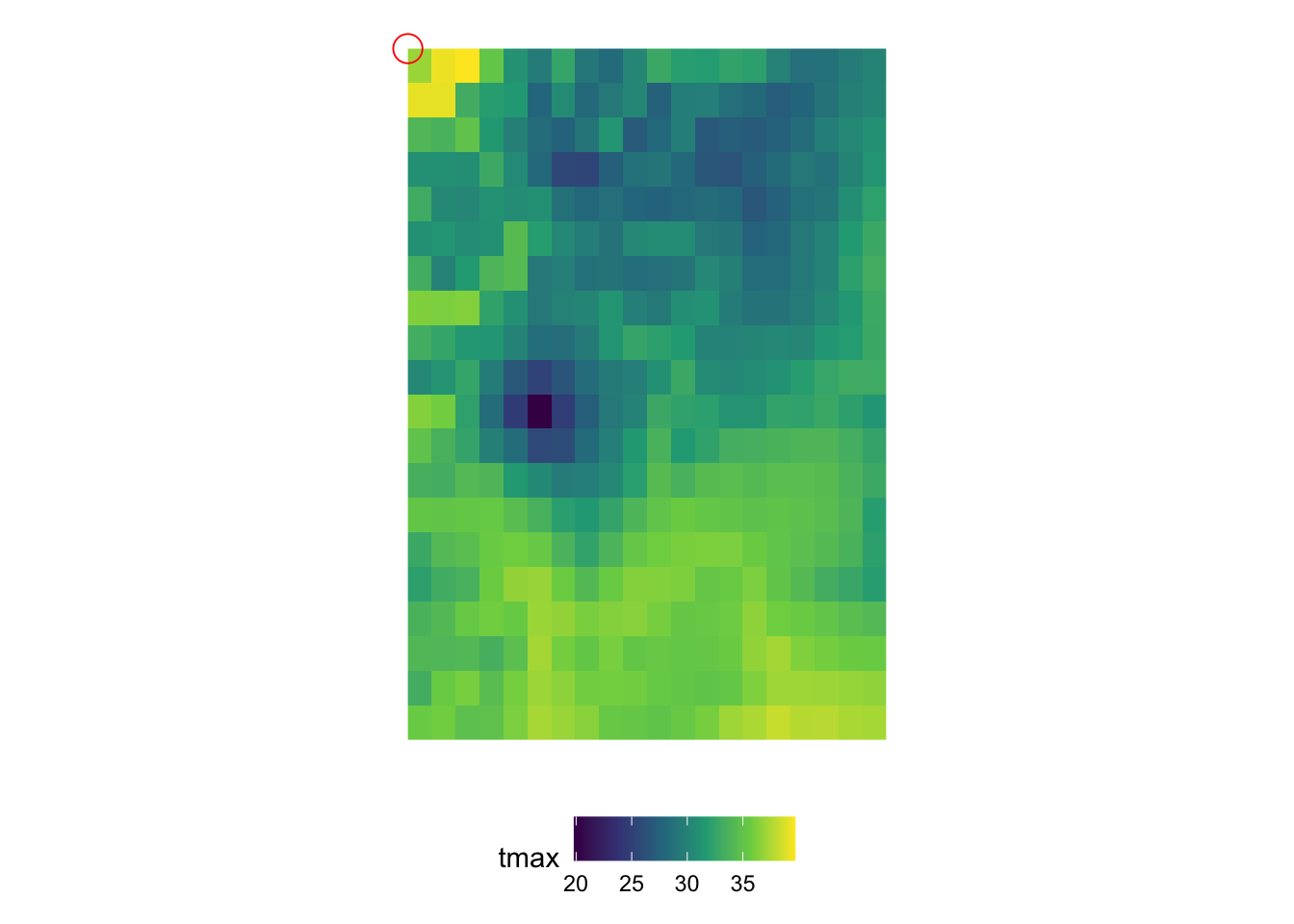
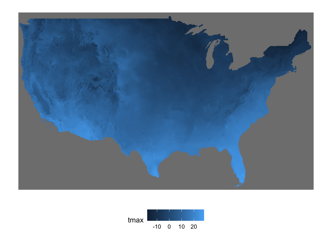
In order to understand the dimensions of stars objects, let’s first take a look at the figure below (Figure 6.1), which visualizes the tmax values on the 2D x-y surfaces of the stars objects at 10th date value (the spatial distribution of tmax at a particular date).
Figure 6.1: Map of tmax values on August 10, 2009: 20 by 20 matrix of cells
You can consider the 2D x-y surface as a matrix, where the location of a cell is defined by the row number and column number. Since the from for x is 1 and to for x is 20, we have 20 columns. Similarly, since the from for y is 1 and to for y is 20, we have 20 rows. The offset value of the x and y dimensions is the longitude and latitude of the upper-left corner point of the upper left cell of the 2D x-y surface, respectively (the red circle i@fig-two-d-map).2 As refsys indicates, they are in NAD83 GCS. The longitude of the upper-left corner point of all the cells in the \(j\)th column (from the left) of the 2D x-y surface is -121.7291667 + \((j-1)\times\) 0.0416667, where -121.7291667 is offset for x and 0.0416667 is delta for x. Similarly, the latitude of the upper-left corner point of all the cells in the \(i\)th row (from the top) of the 2D x-y surface is 46.6458333 +\((i-1)\times\) -0.0416667, where 46.6458333 is offset for y and -0.0416667 is delta for y.
2 This changes depending on the delta of x and y. If both of the delta for x and y are positive, then the offset value of the x and y dimensions are the longitude and latitude of the upper-left corner point of the lower-left cell of the 2D x-y surface.
The dimension characteristics of x and y are shared by all the layers across the date dimension, and a particular combination of x and y indexes refers to exactly the same location on the earth in all the layers across dates (of course). In the date dimension, we have 10 date values since the from for date is 1 and to for date is 10. The refsys of the date dimension is Date. Since the offset is 2009-08-11 and delta is 1, \(k\)th layer represents tmax values for August \(11+k-1\), 2009.
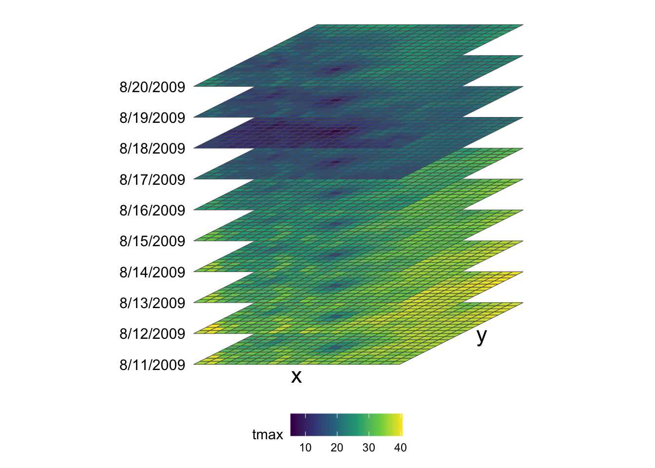
Putting all this information together, we have 20 by 20 x-y surfaces stacked over the date dimension (10 layers), thus making up a 20 by 20 by 10 three-dimensional array (or cube) as shown in the figure below (Figure 6.2).
Figure 6.2: Visual illustration of stars data structure
Remember that prcp_tmax_PRISM_m8_y09 also has another attribute (ppt) which is structured exactly the same way as tmax. So, prcp_tmax_PRISM_m8_y09 basically has four dimensions: attribute, x, y, and date.
It is not guaranteed that all the dimensions are regularly spaced or timed. For an irregular dimension, dimension values themselves are stored in values instead of using indexes, offset, and delta to find dimension values. For example, if you observe satellite data with 6-day gaps sometimes and 7-day gaps other times, then the date dimension would be irregular. We will see a made-up example of irregular time dimension in Section 6.5.
6.2 Some basic operations on stars objects
6.2.1 Create a new attribute and drop a attribute
You can add a new attribute to a stars object just like you add a variable to a data.frame.
#--- define a new variable which is tmax - 20 ---#prcp_tmax_PRISM_m8_y09$tmax_less_20<-prcp_tmax_PRISM_m8_y09$tmax-20
As you can see below, prcp_tmax_PRISM_m8_y09 now has tmax_less_20 as an attribute.
prcp_tmax_PRISM_m8_y09
stars object with 3 dimensions and 3 attributes
attribute(s):
                 Min.  1st Qu. Median      Mean  3rd Qu.   Max.
ppt             0.000  0.00000  0.000  1.292334  0.01100 30.851
tmax            1.833 17.55575 21.483 22.035435 26.54275 39.707
tmax_less_20  -18.167 -2.44425  1.483  2.035435  6.54275 19.707
dimension(s):
     from to     offset    delta refsys point x/y
x       1 20     -121.7  0.04167  NAD83 FALSE [x]
y       1 20      46.65 -0.04167  NAD83 FALSE [y]
date    1 10 2009-08-11   1 days   Date    NA
You can drop an attribute by assining NULL to the attribute you want to drop.
stars object with 3 dimensions and 2 attributes
attribute(s):
       Min.  1st Qu. Median      Mean  3rd Qu.   Max.
ppt   0.000  0.00000  0.000  1.292334  0.01100 30.851
tmax  1.833 17.55575 21.483 22.035435 26.54275 39.707
dimension(s):
     from to     offset    delta refsys point x/y
x       1 20     -121.7  0.04167  NAD83 FALSE [x]
y       1 20      46.65 -0.04167  NAD83 FALSE [y]
date    1 10 2009-08-11   1 days   Date    NA
6.2.2 Subset a stars object by index
In order to access the value of an attribute (say ppt) at a particular location at a particular time from the stars object (prcp_tmax_PRISM_m8_y09), you need to tell R that you are interested in the ppt attribute and specify the corresponding index of x, y, and date. Here, is how you get the ppt value of (3, 4) cell at date = 10.
prcp_tmax_PRISM_m8_y09["ppt", 3, 4, 10]
stars object with 3 dimensions and 1 attribute
attribute(s):
     Min. 1st Qu. Median Mean 3rd Qu. Max.
ppt     0       0      0    0       0    0
dimension(s):
     from to     offset    delta refsys point x/y
x       3  3     -121.7  0.04167  NAD83 FALSE [x]
y       4  4      46.65 -0.04167  NAD83 FALSE [y]
date   10 10 2009-08-11   1 days   Date    NA
This is very much similar to accessing a value from a matrix except that we have more dimensions. The first argument selects the attribute of interest, 2nd x, 3rd y, and 4th date.
Of course, you can subset a stars object to access the value of multiple cells like this:
prcp_tmax_PRISM_m8_y09["ppt", 3:6, 3:4, 5:10]
stars object with 3 dimensions and 1 attribute
attribute(s):
     Min. 1st Qu. Median     Mean 3rd Qu.  Max.
ppt     0       0      0 0.043125       0 0.546
dimension(s):
     from to     offset    delta refsys point x/y
x       3  6     -121.7  0.04167  NAD83 FALSE [x]
y       3  4      46.65 -0.04167  NAD83 FALSE [y]
date    5 10 2009-08-11   1 days   Date    NA
6.2.3 Set attribute names
When you read a raster dataset from a GeoTIFF file, the attribute name is the file name by default. So, you will often encounter cases where you want to change the attribute name. You can set the name of attributes using setNames().
Note that the attribute names of prcp_tmax_PRISM_m8_y09 (original datar) have not changed after this operation (just like dplyr::mutate() or other dplyr functions do):
prcp_tmax_PRISM_m8_y09
stars object with 3 dimensions and 2 attributes
attribute(s):
       Min.  1st Qu. Median      Mean  3rd Qu.   Max.
ppt   0.000  0.00000  0.000  1.292334  0.01100 30.851
tmax  1.833 17.55575 21.483 22.035435 26.54275 39.707
dimension(s):
     from to     offset    delta refsys point x/y
x       1 20     -121.7  0.04167  NAD83 FALSE [x]
y       1 20      46.65 -0.04167  NAD83 FALSE [y]
date    1 10 2009-08-11   1 days   Date    NA
If you want to reflect changes in the variable names while keeping the same object name, you need to assign the output of setNames() to the object as follows:
# the codes in the rest of this chapter use "precipitation" and "tmax" as the variables names, not these onesprcp_tmax_PRISM_m8_y09<-setNames(prcp_tmax_PRISM_m8_y09, c("precipitation", "maximum_temp"))
stars object with 4 dimensions and 1 attribute
attribute(s):
Min. 1st Qu. Median Mean 3rd Qu. Max.
ppt.tmax 0 0 11.799 11.66388 21.535 39.707
dimension(s):
from to offset delta refsys point values x/y
x 1 20 -121.7 0.04167 NAD83 FALSE NULL [x]
y 1 20 46.65 -0.04167 NAD83 FALSE NULL [y]
date 1 10 2009-08-11 1 days Date NA NULL
attributes 1 2 NA NA NA NA ppt , tmax
As you can see, the new stars object has an additional dimension called attributes, which represents attributes and has two dimension values: the first for ppt and second for tmax. Now, if you want to access ppt, you can do the following:
prcp_tmax_four[, , , , "ppt"]
stars object with 4 dimensions and 1 attribute
attribute(s):
Min. 1st Qu. Median Mean 3rd Qu. Max.
ppt.tmax 0 0 0 1.292334 0.011 30.851
dimension(s):
from to offset delta refsys point values x/y
x 1 20 -121.7 0.04167 NAD83 FALSE NULL [x]
y 1 20 46.65 -0.04167 NAD83 FALSE NULL [y]
date 1 10 2009-08-11 1 days Date NA NULL
attributes 1 1 NA NA NA NA ppt
We can do this because the merge kept the attribute names as dimension values as you can see in values.
You can revert it back to the original state using base::split(). Since we want the fourth dimension to dissolve,
stars object with 3 dimensions and 2 attributes
attribute(s):
Min. 1st Qu. Median Mean 3rd Qu. Max.
ppt 0.000 0.00000 0.000 1.292334 0.01100 30.851
tmax 1.833 17.55575 21.483 22.035435 26.54275 39.707
dimension(s):
     from to     offset    delta refsys point x/y
x       1 20     -121.7  0.04167  NAD83 FALSE [x]
y       1 20      46.65 -0.04167  NAD83 FALSE [y]
date    1 10 2009-08-11   1 days   Date    NA
6.3 Quick visualization for exploration
You can use plot() to have a quick static map and tmap::mapview() or the tmap package for interactive views.
There are so many formats in which raster data is stored. Some of the common ones include GeoTIFF, netCDF, GRIB. All the available GDAL drivers for reading and writing raster data can be found by the following code:
You can use stars::read_stars() to read a raster data file. It is very unlikely that the raster file you are trying to read is not in one of the supported formats.
For example, you can read a GeoTIFF file as follows:
stars object with 3 dimensions and 1 attribute
attribute(s), summary of first 1e+05 cells:
                        Min. 1st Qu. Median     Mean 3rd Qu.   Max.  NA's
PRISM_ppt_y2009_m1.tif     0       0  0.436 3.543222  3.4925 56.208 60401
dimension(s):
     from   to offset    delta refsys point
x       1 1405   -125  0.04167  NAD83 FALSE
y       1  621  49.94 -0.04167  NAD83 FALSE
band    1   31     NA       NA     NA    NA
                                                                          values
x                                                                           NULL
y                                                                           NULL
band PRISM_ppt_stable_4kmD2_20090101_bil,...,PRISM_ppt_stable_4kmD2_20090131_bil
     x/y
x    [x]
y    [y]
band
This one imports a raw PRISM data stored as a BIL file.
stars object with 2 dimensions and 2 attributes
attribute(s):
                                 Min. 1st Qu. Median     Mean 3rd Qu.   Max.
1_bil/PRISM_tmax_stable_4km...  3.623  25.318 31.596 29.50749  33.735 48.008
2_bil/PRISM_tmax_stable_4km...  0.808  26.505 30.632 29.93235  33.632 47.999
                                  NA's
1_bil/PRISM_tmax_stable_4km...  390874
2_bil/PRISM_tmax_stable_4km...  390874
dimension(s):
  from   to offset    delta refsys x/y
x    1 1405   -125  0.04167  NAD83 [x]
y    1  621  49.94 -0.04167  NAD83 [y]
As you can see, each file becomes an attribute. It is more convenient to have them as layers stacked along the third dimension. To do that you can add along = 3 option as follows:
(prism_tmax_201807_two<-stars::read_stars(files, along =3))
stars object with 3 dimensions and 1 attribute
attribute(s), summary of first 1e+05 cells:
                                 Min. 1st Qu. Median     Mean 3rd Qu.   Max.
PRISM_tmax_stable_4kmD2_201...  4.693 19.5925 23.653 22.05224 24.5945 33.396
                                 NA's
PRISM_tmax_stable_4kmD2_201...  60401
dimension(s):
        from   to offset    delta refsys
x          1 1405   -125  0.04167  NAD83
y          1  621  49.94 -0.04167  NAD83
new_dim    1    2     NA       NA     NA
                                                                                values
x                                                                                 NULL
y                                                                                 NULL
new_dim 1_bil/PRISM_tmax_stable_4kmD2_20180701, 2_bil/PRISM_tmax_stable_4kmD2_20180702
        x/y
x       [x]
y       [y]
new_dim
Note that while the GeoTIFF format (and many other formats) can store multi-band (multi-layer) raster data allowing for an additional dimension beyond x and y, it does not store the values of the dimension like the date dimension we saw in prcp_tmax_PRISM_m8_y09. So, when you read a multi-layer raster data saved as a GeoTIFF, the third dimension of the resulting stars object will always be called band without any explicit time information. On the other hand, netCDF files are capable of storing the time dimension values. So, when you read a netCDF file with valid time dimension, you will have time dimension when it is read.
stars object with 3 dimensions and 1 attribute
attribute(s):
                             Min.  1st Qu. Median     Mean  3rd Qu.   Max.
tmax_m8_y09_from_stars.tif  1.833 17.55575 21.483 22.03543 26.54275 39.707
dimension(s):
     from to offset    delta refsys point x/y
x       1 20 -121.7  0.04167  NAD83 FALSE [x]
y       1 20  46.65 -0.04167  NAD83 FALSE [y]
band    1 10     NA       NA     NA    NA
Notice that the third dimension is now called band and all the date information is lost. The loss of information happened when we saved prcp_tmax_PRISM_m8_y09["tmax",,,] as a GeoTIFF file. One easy way to avoid this problem is to just save a stars object as an R dataset.
#--- save it as an rds file ---#saveRDS(prcp_tmax_PRISM_m8_y09["tmax", , , ], "Data/tmax_m8_y09_from_stars.rds")
#--- read it back ---#readRDS("Data/tmax_m8_y09_from_stars.rds")
stars object with 3 dimensions and 1 attribute
attribute(s):
       Min.  1st Qu. Median     Mean  3rd Qu.   Max.
tmax  1.833 17.55575 21.483 22.03543 26.54275 39.707
dimension(s):
     from to     offset    delta refsys point x/y
x       1 20     -121.7  0.04167  NAD83 FALSE [x]
y       1 20      46.65 -0.04167  NAD83 FALSE [y]
date    1 10 2009-08-11   1 days   Date    NA
As you can see, date information is retained. So, if you are the only one who uses this data or all of your team members use R, then this is a nice solution to the problem. At the moment, it is not possible to use stars::write_stars() to write to a netCDF file that supports the third dimension as time. However, this may not be the case for a long time (See the discussion here).
6.5 Setting the time dimension manually
For this section, we will use PRISM precipitation data for U.S. for January, 2009.
stars object with 3 dimensions and 1 attribute
attribute(s), summary of first 1e+05 cells:
                        Min. 1st Qu. Median     Mean 3rd Qu.   Max.  NA's
PRISM_ppt_y2009_m1.tif     0       0  0.436 3.543222  3.4925 56.208 60401
dimension(s):
     from   to offset    delta refsys point
x       1 1405   -125  0.04167  NAD83 FALSE
y       1  621  49.94 -0.04167  NAD83 FALSE
band    1   31     NA       NA     NA    NA
                                                                          values
x                                                                           NULL
y                                                                           NULL
band PRISM_ppt_stable_4kmD2_20090101_bil,...,PRISM_ppt_stable_4kmD2_20090131_bil
     x/y
x    [x]
y    [y]
band
As you can see, when you read a GeoTIFF file, the third dimension will always be called band because GeoTIFF format does not support dimension values for the third dimension.3
3 In Section 6.1, we read an rds, which is a stars object with dimension name set manually.
You can use st_set_dimension() to set the third dimension (called band) as the time dimension using Date object. This can be convenient when you would like to filter the data by date using filter() as we will see later.
For ppt_m1_y09_stars, precipitation is observed on a daily basis from January 1, 2009 to January 31, 2009, where the band value of x corresponds to January x, 2009. So, we can first create a vector of dates as follows (If you are not familiar with Dates and the lubridate pacakge, this is a good resource to learn them.):
#--- starting date ---#start_date<-lubridate::ymd("2009-01-01")#--- ending date ---#end_date<-lubridate::ymd("2009-01-31")#--- sequence of dates ---#(dates_ls_m1<-seq(start_date, end_date, "days"))
stars object with 3 dimensions and 1 attribute
attribute(s), summary of first 1e+05 cells:
                        Min. 1st Qu. Median     Mean 3rd Qu.   Max.  NA's
PRISM_ppt_y2009_m1.tif     0       0  0.436 3.543222  3.4925 56.208 60401
dimension(s):
     from   to     offset    delta refsys point x/y
x       1 1405       -125  0.04167  NAD83 FALSE [x]
y       1  621      49.94 -0.04167  NAD83 FALSE [y]
date    1   31 2009-01-01   1 days   Date    NA
As you can see, the third dimension has become date. The value of offset for the date dimension has become 2009-01-01 meaning the starting date value is now 2009-01-01. Further, the value of delta is now 1 days, so date dimension of x corresponds to 2009-01-01 + x - 1 = 2009-01-x.
Note that the date dimension does not have to be regularly spaced. For example, you may have satellite images available for your area with a 5-day interval sometimes and a 6-day interval other times. This is perfectly fine. As an illustration, I will create a wrong sequence of dates for this data with a 2-day gap in the middle and assign them to the date dimension to see what happens.
#--- 2009-01-23 removed and 2009-02-01 added ---#(dates_ls_wrong<-c(seq(start_date, end_date, "days")[-23], lubridate::ymd("2009-02-01")))
#--- set date values ---#(ppt_m1_y09_stars_wrong<-stars::st_set_dimensions(ppt_m1_y09_stars,3, values =dates_ls_wrong, names ="date"))
stars object with 3 dimensions and 1 attribute
attribute(s), summary of first 1e+05 cells:
                        Min. 1st Qu. Median     Mean 3rd Qu.   Max.  NA's
PRISM_ppt_y2009_m1.tif     0       0  0.436 3.543222  3.4925 56.208 60401
dimension(s):
     from   to offset    delta refsys point                    values x/y
x       1 1405   -125  0.04167  NAD83 FALSE                      NULL [x]
y       1  621  49.94 -0.04167  NAD83 FALSE                      NULL [y]
date    1   31     NA       NA   Date    NA 2009-01-01,...,2009-02-01
Since the step between the date values is no longer \(1\) day for the entire sequence, the value of delta is now NA. However, notice that the value of date is no longer NULL. Since the date is not regular, you cannot represent date using three values (from, to, and delta) any more, and date values for each observation have to be stored now.
Finally, note that just applying stars::st_set_dimensions() to a stars object does not change the dimension of the stars object (just like setNames() as we discussed above).
ppt_m1_y09_stars
stars object with 3 dimensions and 1 attribute
attribute(s), summary of first 1e+05 cells:
                        Min. 1st Qu. Median     Mean 3rd Qu.   Max.  NA's
PRISM_ppt_y2009_m1.tif     0       0  0.436 3.543222  3.4925 56.208 60401
dimension(s):
     from   to     offset    delta refsys point x/y
x       1 1405       -125  0.04167  NAD83 FALSE [x]
y       1  621      49.94 -0.04167  NAD83 FALSE [y]
date    1   31 2009-01-01   1 days   Date    NA
As you can see, the date dimension has not been altered. You need to assign the results of stars::st_set_dimensions() to a stars object to see the changes in the dimension reflected just like we did above with the right date values.
6.6dplyr-like operations
You can use the dplyr language to do basic data operations on stars objects.
6.6.1dplyr::filter()
The dplyr::filter() function allows you to subset data by dimension values: x, y, and band (here date).
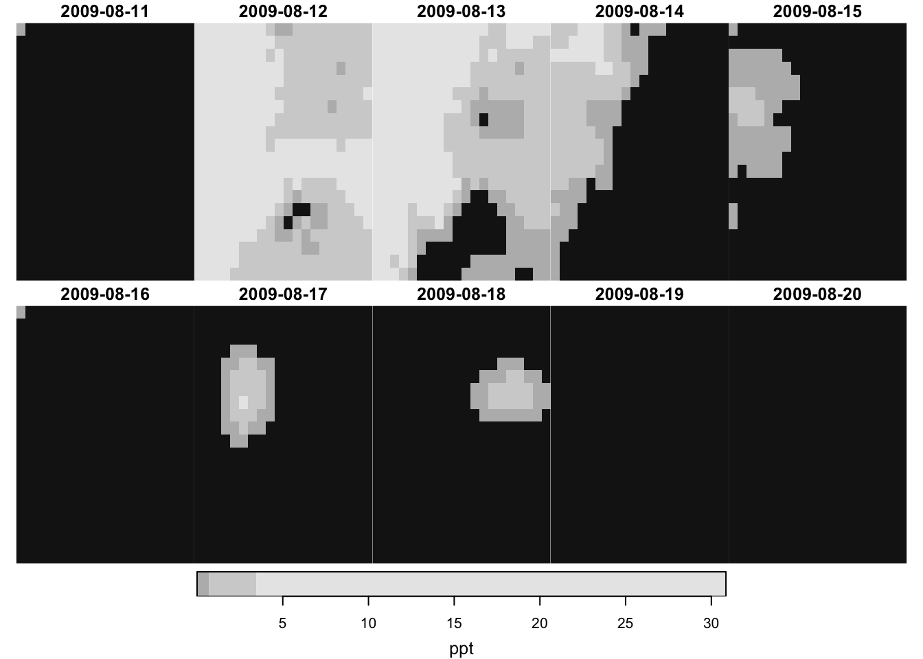
spatial filtering
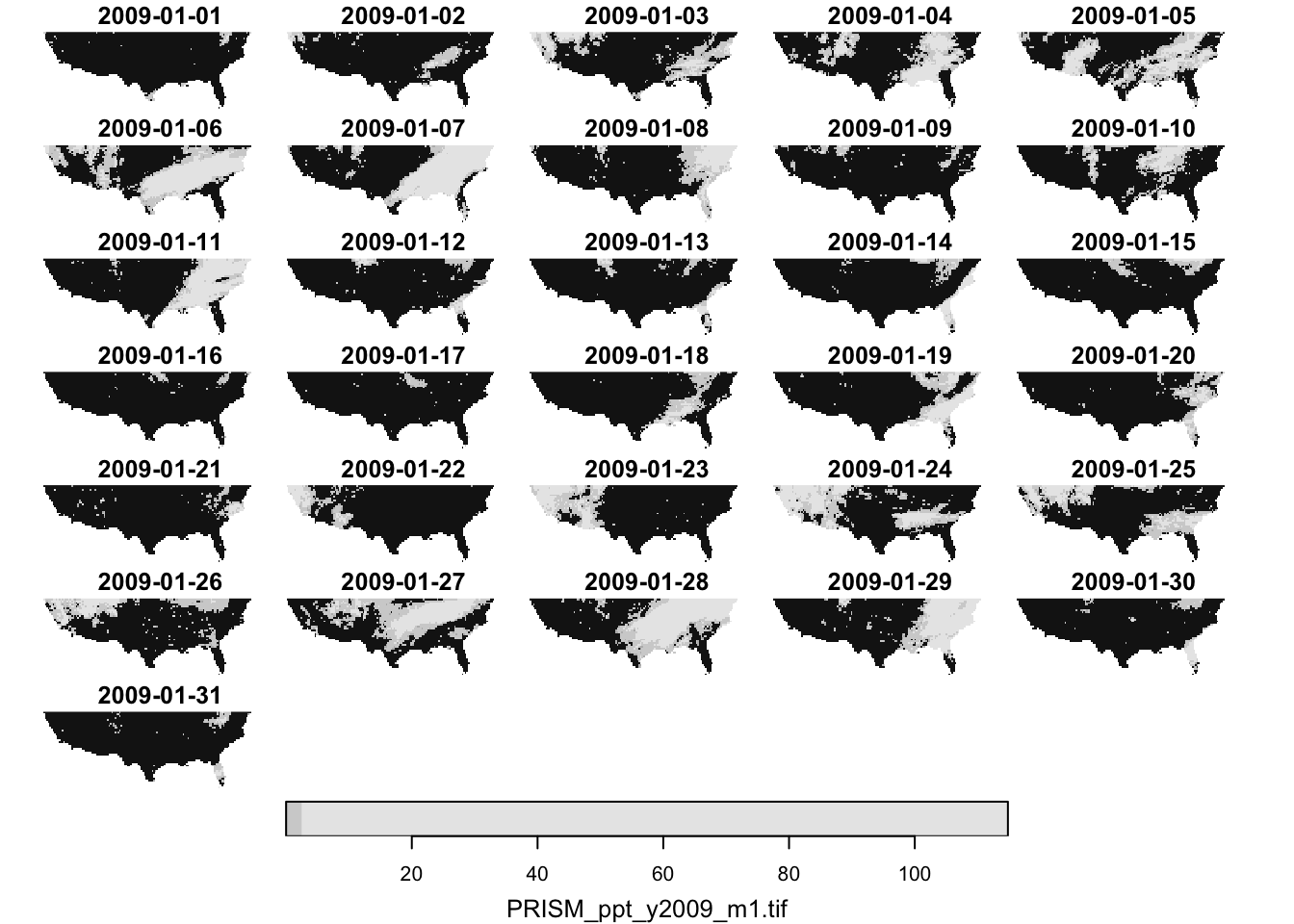
#--- longitude greater than -100 ---#dplyr::filter(ppt_m1_y09_stars, x>-100)%>%plot()
#--- latitude less than 40 ---#dplyr::filter(ppt_m1_y09_stars, y<40)%>%plot()
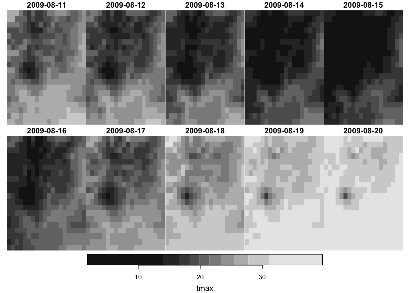
temporal filtering
Finally, since the date dimension is in Date, you can use Date math to filter the data.4
4 This is possible only because we have assigned date values to the band dimension above.
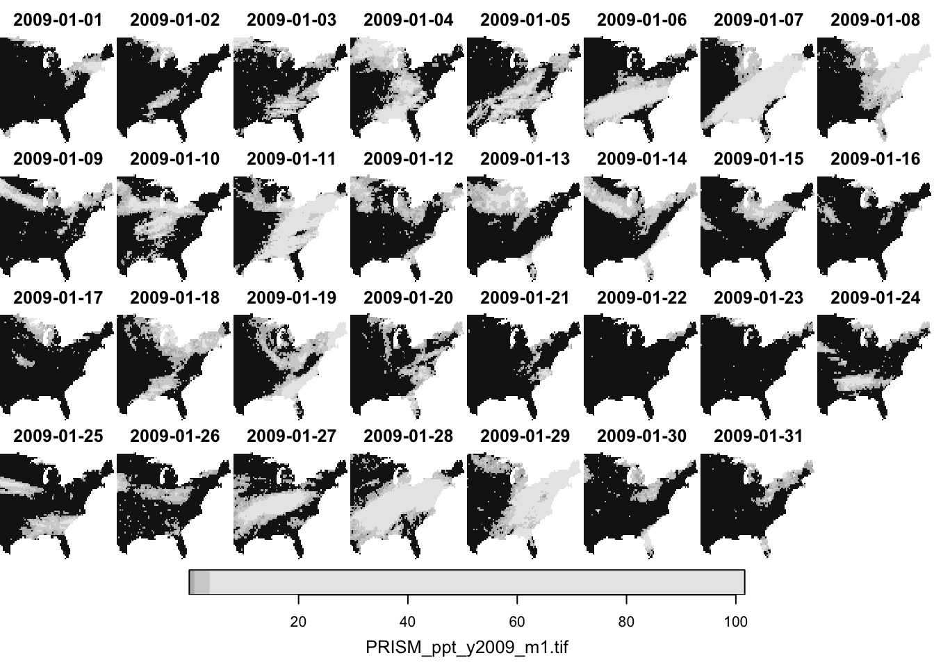
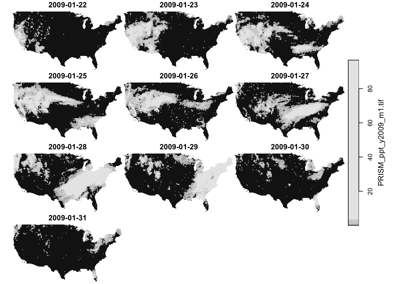
#--- dates after 2009-01-15 ---#dplyr::filter(ppt_m1_y09_stars, date>lubridate::ymd("2009-01-21"))%>%plot()
filter by attribute?
In case you are wondering, filtering by attribute is not possible. This makes sense, as doing so would disrupt the regular grid structure of raster data.
stars object with 3 dimensions and 1 attribute
attribute(s):
     Min. 1st Qu. Median     Mean 3rd Qu.   Max.
ppt     0       0      0 1.292334   0.011 30.851
dimension(s):
     from to     offset    delta refsys point x/y
x       1 20     -121.7  0.04167  NAD83 FALSE [x]
y       1 20      46.65 -0.04167  NAD83 FALSE [y]
date    1 10 2009-08-11   1 days   Date    NA
6.6.3dplyr::mutate()
You can mutate attributes using the dplyr::mutate() function. For example, this can be useful to calculate NDVI in a stars object that has Red and NIR (spectral reflectance measurements in the red and near-infrared regions) as attributes. Here, we just simply convert the unit of precipitation from mm to inches.
#--- mm to inches ---#dplyr::mutate(prcp_tmax_PRISM_m8_y09, ppt =ppt*0.0393701)
stars object with 3 dimensions and 2 attributes
attribute(s):
       Min.  1st Qu. Median       Mean      3rd Qu.      Max.
ppt   0.000  0.00000  0.000  0.0508793 4.330711e-04  1.214607
tmax  1.833 17.55575 21.483 22.0354348 2.654275e+01 39.707001
dimension(s):
     from to     offset    delta refsys point x/y
x       1 20     -121.7  0.04167  NAD83 FALSE [x]
y       1 20      46.65 -0.04167  NAD83 FALSE [y]
date    1 10 2009-08-11   1 days   Date    NA
6.6.4dplyr::pull()
You can extract attribute values using dplyr::pull().
#--- tmax values of the 1st date layer ---#dplyr::pull(prcp_tmax_PRISM_m8_y09["tmax", , , 1], "tmax")
6.7 Merging stars objects using c() and stars::st_mosaic()
6.7.1 Merging stars objects along the third dimension (band)
Here we learn how to merge multiple stars objects that have
the same attributes
the same spatial extent and resolution
different bands (dates here)
For example, consider merging PRISM precipitation data in January and February. Both of them have exactly the same spatial extent and resolutions and represent the same attribute (precipitation). However, they differ in the third dimension (date). So, you are trying to stack data of the same attributes along the third dimension (date) while making sure that spatial correspondence is maintained. This merge is kind of like rbind() that stacks multiple data.frames vertically while making sure the variables are aligned correctly.
Let’s import the PRISM precipitation data for February, 2009.
#--- read the February ppt data ---#(ppt_m2_y09_stars<-stars::read_stars("Data/PRISM_ppt_y2009_m2.tif"))
stars object with 3 dimensions and 1 attribute
attribute(s), summary of first 1e+05 cells:
                        Min. 1st Qu. Median      Mean 3rd Qu.   Max.  NA's
PRISM_ppt_y2009_m2.tif     0       0      0 0.1855858       0 11.634 60401
dimension(s):
     from   to offset    delta refsys point
x       1 1405   -125  0.04167  NAD83 FALSE
y       1  621  49.94 -0.04167  NAD83 FALSE
band    1   28     NA       NA     NA    NA
                                                                          values
x                                                                           NULL
y                                                                           NULL
band PRISM_ppt_stable_4kmD2_20090201_bil,...,PRISM_ppt_stable_4kmD2_20090228_bil
     x/y
x    [x]
y    [y]
band
Note here that the third dimension of ppt_m2_y09_stars has not been changed to date.
Now, let’s try to merge the two:
#--- combine the two ---#(ppt_m1_to_m2_y09_stars<-c(ppt_m1_y09_stars, ppt_m2_y09_stars, along =3))
stars object with 3 dimensions and 1 attribute
attribute(s), summary of first 1e+05 cells:
                        Min. 1st Qu. Median     Mean 3rd Qu.   Max.  NA's
PRISM_ppt_y2009_m1.tif     0       0  0.436 3.543222  3.4925 56.208 60401
dimension(s):
     from   to     offset    delta refsys point x/y
x       1 1405       -125  0.04167  NAD83 FALSE [x]
y       1  621      49.94 -0.04167  NAD83 FALSE [y]
date    1   59 2009-01-01   1 days   Date    NA
As you noticed, the second object (ppt_m2_y09_stars) was assumed to have the same date characteristics as the first one: the data in February is observed daily (delta is 1 day). This causes no problem in this instance as the February data is indeed observed daily starting from 2009-02-01. However, be careful if you are appending the data that does not start from 1 day after (or more generally delta for the time dimension) the first data or the data that does not follow the same observation interval.
For this reason, it is advisable to first set the date values if it has not been set. Pretend that the February data actually starts from 2009-02-02 to 2009-03-01 to see what happens when the regular interval (delta) is not kept after merging.
#--- starting date ---#start_date<-lubridate::ymd("2009-02-01")#--- ending date ---#end_date<-lubridate::ymd("2009-02-28")#--- sequence of dates ---#dates_ls<-seq(start_date, end_date, "days")#--- pretend the data actually starts from `2009-02-02` to `2009-03-01` ---#(ppt_m2_y09_stars<-stars::st_set_dimensions(ppt_m2_y09_stars,3, values =c(dates_ls[-1], lubridate::ymd("2009-03-01")), name ="date"))
stars object with 3 dimensions and 1 attribute
attribute(s), summary of first 1e+05 cells:
                        Min. 1st Qu. Median      Mean 3rd Qu.   Max.  NA's
PRISM_ppt_y2009_m2.tif     0       0      0 0.1855858       0 11.634 60401
dimension(s):
     from   to     offset    delta refsys point x/y
x       1 1405       -125  0.04167  NAD83 FALSE [x]
y       1  621      49.94 -0.04167  NAD83 FALSE [y]
date    1   28 2009-02-02   1 days   Date    NA
stars object with 3 dimensions and 1 attribute
attribute(s), summary of first 1e+05 cells:
                        Min. 1st Qu. Median     Mean 3rd Qu.   Max.  NA's
PRISM_ppt_y2009_m1.tif     0       0  0.436 3.543222  3.4925 56.208 60401
dimension(s):
     from   to offset    delta refsys point                    values x/y
x       1 1405   -125  0.04167  NAD83 FALSE                      NULL [x]
y       1  621  49.94 -0.04167  NAD83 FALSE                      NULL [y]
date    1   59     NA       NA   Date    NA 2009-01-01,...,2009-03-01
The date dimension does not have delta any more, and correctly so because there is a one-day gap between the end date of the first stars object ("2009-01-31") and the start date of the second stars object ("2009-02-02"). So, all the date values are now stored in values.
6.7.2 Merging stars objects of different attributes
Here we learn how to merge multiple stars objects that have
different attributes
the same spatial extent and resolution
the same bands (dates here)
For example, consider merging PRISM precipitation and tmax data in January. Both of them have exactly the same spatial extent and resolutions and the date characteristics (starting and ending on the same dates with the same time interval). However, they differ in what they represent: precipitation and tmax. This merge is kind of like cbind() that combines multiple data.frames of different variables while making sure the observation correspondence is correct.
Let’s read the daily tmax data for January, 2009:
(tmax_m8_y09_stars<-stars::read_stars("Data/PRISM_tmax_y2009_m1.tif")%>%#--- change the attribute name ---#setNames("tmax"))
stars object with 3 dimensions and 1 attribute
attribute(s), summary of first 1e+05 cells:
         Min. 1st Qu. Median      Mean 3rd Qu.  Max.  NA's
tmax  -17.898  -7.761 -2.248 -3.062721   1.718 7.994 60401
dimension(s):
     from   to offset    delta refsys point
x       1 1405   -125  0.04167  NAD83 FALSE
y       1  621  49.94 -0.04167  NAD83 FALSE
band    1   31     NA       NA     NA    NA
                                                                            values
x                                                                             NULL
y                                                                             NULL
band PRISM_tmax_stable_4kmD2_20090101_bil,...,PRISM_tmax_stable_4kmD2_20090131_bil
     x/y
x    [x]
y    [y]
band
Now, let’s merge the PRISM ppt and tmax data in January, 2009.
Error in c.stars(ppt_m1_y09_stars, tmax_m8_y09_stars): don't know how to merge arrays: please specify parameter along
Oops. Well, the problem is that the third dimension of the two objects is not the same. Even though we know that the xth element of their third dimension represent the same thing, they look different to R’s eyes. So, we first need to change the third dimension of tmax_m8_y09_stars to be consistent with the third dimension of ppt_m1_y09_stars (dates_ls_m1 was defined in Section 6.5).
stars object with 3 dimensions and 1 attribute
attribute(s), summary of first 1e+05 cells:
         Min. 1st Qu. Median      Mean 3rd Qu.  Max.  NA's
tmax  -17.898  -7.761 -2.248 -3.062721   1.718 7.994 60401
dimension(s):
     from   to     offset    delta refsys point x/y
x       1 1405       -125  0.04167  NAD83 FALSE [x]
y       1  621      49.94 -0.04167  NAD83 FALSE [y]
date    1   31 2009-01-01   1 days   Date    NA
stars object with 3 dimensions and 2 attributes
attribute(s), summary of first 1e+05 cells:
                           Min. 1st Qu. Median      Mean 3rd Qu.   Max.  NA's
PRISM_ppt_y2009_m1.tif    0.000   0.000  0.436  3.543222  3.4925 56.208 60401
tmax                    -17.898  -7.761 -2.248 -3.062721  1.7180  7.994 60401
dimension(s):
     from   to     offset    delta refsys point x/y
x       1 1405       -125  0.04167  NAD83 FALSE [x]
y       1  621      49.94 -0.04167  NAD83 FALSE [y]
date    1   31 2009-01-01   1 days   Date    NA
As you can see, now we have another attribute called tmax.
6.7.3 Merging stars objects of different spatial extents
Here we learn how to merge multiple stars objects that have
5 Technically, you can actually merge stars objects of different spatial resolutions. But, you probably should not.
Some times you have multiple separate raster datasets that have different spatial coverages and would like to combine them into one. You can do that using stars::st_mosaic().
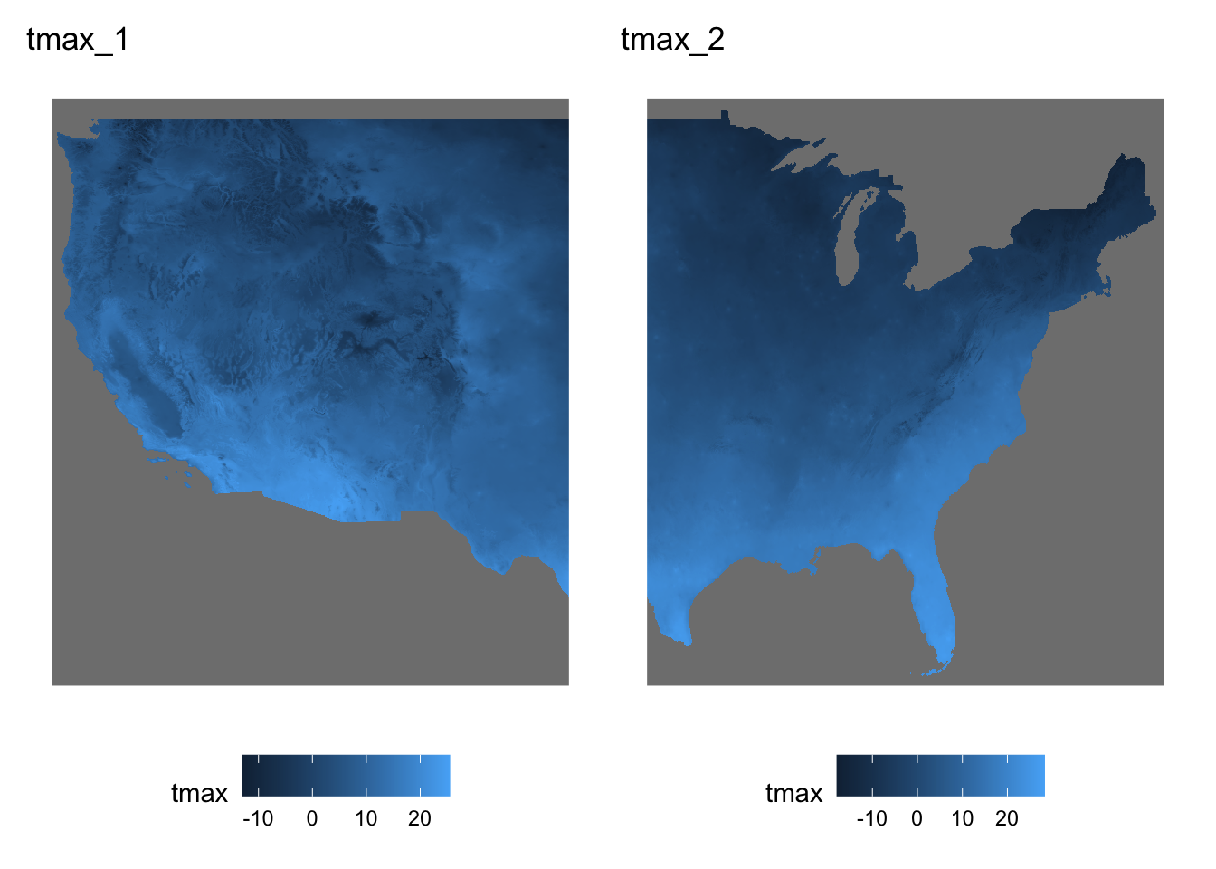
Let’s split tmax_m8_y09_stars into two parts (Figure 6.3 shows what they look like (only Jan 1, 1980)):
Figure 6.4: Map of the stars objects combined into one
It is okay to have the two stars objects to be combined have a spatial overlap. The following split creates two stars objects with a spatial overlap (Figure 6.5 shows what they look like).
stars object with 3 dimensions and 1 attribute
attribute(s), summary of first 1e+05 cells:
         Min. 1st Qu. Median      Mean 3rd Qu.  Max.  NA's
tmax  -17.898  -7.761 -2.248 -3.062721   1.718 7.994 60401
dimension(s):
     from   to offset    delta refsys x/y
x       1 1405   -125  0.04167  NAD83 [x]
y       1  621  49.94 -0.04167  NAD83 [y]
band    1   31     NA       NA     NA
Figure 6.6: Map of the spatially-overlapping stars objects combined into one
6.8 Apply a function to one or more dimensions
At times, you may want to apply a function to one or more dimensions of a stars object. For instance, you might want to calculate the total annual precipitation for each cell using daily precipitation data. To illustrate this, let’s create a single-attribute stars object that contains daily precipitation data for August 2009.
(ppt_m8_y09<-prcp_tmax_PRISM_m8_y09["ppt"])
stars object with 3 dimensions and 1 attribute
attribute(s):
     Min. 1st Qu. Median     Mean 3rd Qu.   Max.
ppt     0       0      0 1.292334   0.011 30.851
dimension(s):
     from to     offset    delta refsys point x/y
x       1 20     -121.7  0.04167  NAD83 FALSE [x]
y       1 20      46.65 -0.04167  NAD83 FALSE [y]
date    1 10 2009-08-11   1 days   Date    NA
Let’s find total precipitation for each cell in August in 2009 using stars::st_apply(), which works like this.
stars::st_apply(X = stars object,MARGIN = margin,FUN =function to apply)
Since we want to sum the value of attribute (ppt) for each of the cells (each cell is represented by x-y), we specify MARGIN = c("x", "y") and use sum() as the function (Figure 6.7 shows the results).
monthly_ppt<-stars::st_apply(ppt_m8_y09, MARGIN =c("x", "y"), FUN =sum)
As you can see, date values in prcp_tmax_PRISM_m8_y09 appear in the time dimension of prcp_tmax_PRISM_m8_y09_rb (RasterBrick). However, in prcp_tmax_PRISM_m8_y09_sr (SpatRaster), date values appear in the names dimension with date added as prefix to the original date values.
Note also that the conversion was done for only the ppt attribute. This is simply because the raster and terra package does not accommodate multiple attributes of 3-dimensional array. So, if you want a RasterBrick or SpatRaster of the precipitation data, then you need to do the following:
(# to RasterBricktmax_PRISM_m8_y09_rb<-as(prcp_tmax_PRISM_m8_y09["ppt", , , ], "Raster"))
stars object with 3 dimensions and 1 attribute
attribute(s):
         Min. 1st Qu. Median     Mean 3rd Qu.   Max.
layer.1     0       0      0 1.292334   0.011 30.851
dimension(s):
     from to     offset    delta refsys x/y
x       1 20     -121.7  0.04167  NAD83 [x]
y       1 20      46.65 -0.04167  NAD83 [y]
band    1 10 2009-08-11   1 days   Date
Notice that the original date values (stored in the date dimension) are recovered, but its dimension is now called just band.
stars object with 3 dimensions and 1 attribute
attribute(s):
       Min. 1st Qu. Median     Mean 3rd Qu.   Max.
lyr.1     0       0      0 1.292334   0.011 30.851
dimension(s):
     from to     offset    delta refsys x/y
x       1 20     -121.7  0.04167  NAD83 [x]
y       1 20      46.65 -0.04167  NAD83 [y]
time    1 10 2009-08-11   1 days   Date
Note that unlike the conversion from the RasterBrick object, the band dimension inherited values of the name dimension in tmax_PRISM_m8_y09_sr.
6.10 Spatial interactions of stars and sf objects
6.10.1 Spatial cropping (subsetting) to the area of interest
If the region of interest is smaller than the spatial extent of the stars raster data, there is no need to retain the irrelevant portions of the stars object. In such cases, you can crop the stars data to focus on the region of interest using sf::st_crop(). The general syntax of sf::st_crop() is:
#--- NOT RUN ---#sf::st_crop(stars object, sf/bbox object)
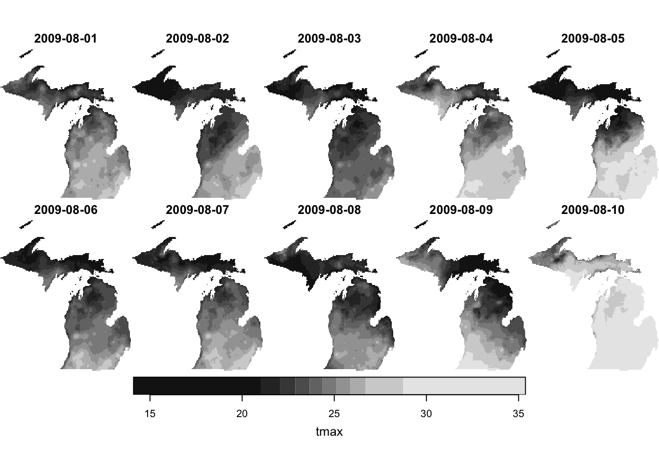
For demonstration, we use PRISM tmax data for the U.S. for January 2019 as a stars object.
(tmax_m8_y09_stars<-stars::read_stars("Data/PRISM_tmax_y2009_m8.tif")%>%setNames("tmax")%>%.[, , , 1:10]%>%stars::st_set_dimensions("band", values =seq(lubridate::ymd("2009-08-01"),lubridate::ymd("2009-08-10"), by ="days"), name ="date"))
stars object with 3 dimensions and 1 attribute
attribute(s), summary of first 1e+05 cells:
        Min. 1st Qu. Median     Mean 3rd Qu.   Max.  NA's
tmax  15.084 20.1775 22.584 23.86903 26.3285 41.247 60401
dimension(s):
     from   to     offset    delta refsys point x/y
x       1 1405       -125  0.04167  NAD83 FALSE [x]
y       1  621      49.94 -0.04167  NAD83 FALSE [y]
date    1   10 2009-08-01   1 days   Date    NA
The region of interest is Michigan.
MI_county_sf<-tigris::counties(state ="Michigan", cb =TRUE, progress_bar =FALSE)%>%#--- transform using the CRS of the PRISM stars data ---#sf::st_transform(sf::st_crs(tmax_m8_y09_stars))
We can crop the tmax data to the Michigan state border using st_crop() as follows:
stars object with 3 dimensions and 1 attribute
attribute(s):
        Min. 1st Qu. Median     Mean 3rd Qu.   Max.   NA's
tmax  14.108  22.471 24.343 24.61851  26.208 35.373 206900
dimension(s):
     from   to     offset    delta refsys point x/y
x     831 1023       -125  0.04167  NAD83 FALSE [x]
y      41  198      49.94 -0.04167  NAD83 FALSE [y]
date    1   10 2009-08-01   1 days   Date    NA
Notice that from and to for x and y have changed to cover only the boundary box of the Michigan state border. Note that the values for the cells outside of the Michigan state border were set to NA. Figure 6.8 shows the cropping was successful.
When using sf::st_crop(), it is much faster to crop to a bounding box instead of sf if that is satisfactory. For example, you may be cropping a stars object to speed up subsequent raster value extraction (see Section 9.2). In this case, it is far better to crop to the bounding box of the sf instead of sf. Confirm the speed difference between the two below:
The difference can be substantial especially when the number of observations are large in sf.
6.10.2 Extracting values for points
In this section, we will learn how to extract cell values from raster layers as starts for spatial units represented as point sf data6.
6 see Section 5.2 for a detailed explanation of what it means to extract raster values.
6.10.2.1 Extraction using stars::st_extract()
For the illustrations in this section, we use the following datasets:
Points: Irrigation wells in Kansas
Raster: daily PRISM tmax data for August, 2009
PRISM tmax data
(tmax_m8_y09_stars<-stars::read_stars("Data/PRISM_tmax_y2009_m8.tif")%>%setNames("tmax")%>%.[, , , 1:10]%>%stars::st_set_dimensions("band", values =seq(lubridate::ymd("2009-08-01"),lubridate::ymd("2009-08-10"), by ="days"), name ="date"))
Irrigation wells in Kansas:
#--- read in the KS points data ---#(KS_wells<-readRDS("Data/Chap_5_wells_KS.rds"))
Simple feature collection with 37647 features and 1 field
Geometry type: POINT
Dimension:     XY
Bounding box:  xmin: -102.0495 ymin: 36.99552 xmax: -94.62089 ymax: 40.00199
Geodetic CRS:  NAD83
First 10 features:
   well_id                   geometry
1        1 POINT (-100.4423 37.52046)
2        3 POINT (-100.7118 39.91526)
3        5 POINT (-99.15168 38.48849)
4        7 POINT (-101.8995 38.78077)
5        8  POINT (-100.7122 38.0731)
6        9 POINT (-97.70265 39.04055)
7       11 POINT (-101.7114 39.55035)
8       12 POINT (-95.97031 39.16121)
9       15 POINT (-98.30759 38.26787)
10      17 POINT (-100.2785 37.71539)
Figure 6.9 show the spatial distribution of the irrigation wells over the PRISM grids:
stars object with 2 dimensions and 1 attribute
attribute(s):
        Min. 1st Qu. Median     Mean  3rd Qu.   Max.
tmax  24.605  30.681  33.08 33.22354 36.38175 40.759
dimension(s):
         from    to     offset  delta refsys point
geometry    1 37647         NA     NA  NAD83  TRUE
date        1    10 2009-08-01 1 days   Date    NA
                                                            values
geometry POINT (-100.4423 37.52046),...,POINT (-99.96733 39.88535)
date                                                          NULL
The returned object is a stars object of simple features. You can convert this to a more familiar-looking sf object using sf::st_as_sf():
As you can see each date forms a column of extracted values for the points because the third dimension of tmax_MI is date. So, you can easily turn the outcome to an sf object with date as Date object as follows.
Note that all the variables other than geometry in the points data (KS_wells) are lost at the time of applying stars::st_extract(). You take advantage the fact that the the order of the observations in the object returned by stars::st_extract() is the order of the points (KS_wells).
We can now summarize the data by well_id and then merge it back to KS_wells.
KS_wells<-extracted_tmax_long%>%#--- geometry no longer needed ---## if you do not do this, summarize() takes a long timesf::st_drop_geometry()%>%dplyr::group_by(well_id, month(date))%>%dplyr::summarize(mean(tmax))%>%dplyr::left_join(KS_wells, ., by ="well_id")
6.10.3 Extract and summarize values for polygons
In this section, we will learn how to extract cell values from raster layers as starts for spatial units represented as polygons sf data (see Section 5.2 for a more detailed explanation of this operation).
In order to extract cell values from stars objects (just like Chapter 5) and summarize them for polygons, you can use aggregate.stars(). Although introduced here because it natively accepts stars objects, aggregate.stars() is not recommended unless the raster data is small (with a small number of cells). It is almost always slower than the two other alternatives: terra::extract() and exactextractr::exact_extract() even though they involve conversion of stars objects to SpatRaster objects. For a comparison of its performance relative to these alternatives, see Section 9.3. If you just want to see the better alternatives, you can just skip to Section 6.10.3.2.
6.10.3.1aggregate.stars()
The syntax of aggregate.stars() is as follows:
#--- NOT RUN ---#aggregate(stars object, sf object, FUN =function to apply)
For each polygon, aggregate() identifies the cells whose centroids lie within the polygon, extracts their values, and applies the specified function to those values. Let’s now see a demonstration of how to use aggregate(). For this example, we will use Kansas counties as the polygon data.
KS_county_sf<-tigris::counties(state ="Kansas", cb =TRUE, progress_bar =FALSE)%>%#--- transform using the CRS of the PRISM stars data ---#sf::st_transform(sf::st_crs(tmax_m8_y09_stars))%>%#--- generate unique id ---#dplyr::mutate(id =1:nrow(.))
Figure 6.10 shows polygons (counties) superimposed on top of the tmax raster data:
Code
ggplot()+geom_stars(data =sf::st_crop(tmax_m8_y09_stars, sf::st_bbox(KS_county_sf))[,,,1])+scale_fill_viridis()+geom_sf(data =KS_county_sf, fill =NA)+theme_void()
Figure 6.10: Map of Kansas counties over tmax raster data
For example, the following code will find the mean of the tmax values for each county:
(mean_tmax_stars<-aggregate(tmax_m8_y09_stars, KS_county_sf, FUN =mean))
stars object with 2 dimensions and 1 attribute
attribute(s):
          Min.  1st Qu.   Median    Mean  3rd Qu.     Max.
tmax  24.91317 29.65889 32.56404 32.5487 35.34826 39.70888
dimension(s):
         from  to     offset  delta refsys point
geometry    1 105         NA     NA  NAD83 FALSE
date        1  10 2009-08-01 1 days   Date    NA
                                                                values
geometry MULTIPOLYGON (((-95.52265...,...,MULTIPOLYGON (((-99.0327 ...
date                                                              NULL
As you can see, the aggregate() operation also returns a stars object for polygons just like stars::st_extract() did. You can convert the stars object into an sf object using sf::st_as_sf():
As you can see, aggregate() function extracted values for the polygons from all the layers across the date dimension, and the values from individual dates become variables where the variables names are the corresponding date values.
Just like the case of raster data extraction for points data we saw in Section 6.10.2, no information from the polygons (KS_county_sf) except the geometry column remains. For further processing of the extracted data and easy merging with the polygons data (KS_county_sf), we can assign the unique county id just like we did for the case of points data.
(mean_tmax_long<-mean_tmax_sf%>%#--- drop geometry ---#sf::st_drop_geometry()%>%#--- assign id before transformation ---#dplyr::mutate(id =KS_county_sf$id)%>%#--- then transform ---#tidyr::pivot_longer(-id, names_to ="date", values_to ="tmax"))
aggregate() will return NA for polygons that intersect with raster cells that have NA values. To ignore the NA values when applying a function, we can add na.rm=TRUE option like this:
(mean_tmax_stars<-aggregate(tmax_m8_y09_stars,KS_county_sf, FUN =mean, na.rm =TRUE)%>%sf::st_as_sf())
6.10.3.2exactextractr::exact_extract()
A great alternative to aggregate() is to extract raster cell values using exactextractr::exact_extract() or terra::extract() and then summarize the results yourself. Both are considerably faster than aggregate.stars(). Although they do not natively accept stars objects, you can easily convert a stars object to a SpatRaster using as(stars, "SpatRaster") and then use these methods.
Let’s first convert tmax_m8_y09_KS_stars (a stars object) into a SpatRaster object.
[[1]]
  COUNTYFP lyr.1 lyr.2 lyr.3 lyr.4 lyr.5 lyr.6 lyr.7 lyr.8 lyr.9 lyr.10
1      099    NA    NA    NA    NA    NA    NA    NA    NA    NA     NA
2      099    NA    NA    NA    NA    NA    NA    NA    NA    NA     NA
3      099    NA    NA    NA    NA    NA    NA    NA    NA    NA     NA
4      099    NA    NA    NA    NA    NA    NA    NA    NA    NA     NA
5      099    NA    NA    NA    NA    NA    NA    NA    NA    NA     NA
6      099    NA    NA    NA    NA    NA    NA    NA    NA    NA     NA
  coverage_fraction
1      0.0007206142
2      0.7114530802
3      0.7162888646
4      0.7163895965
5      0.7166024446
6      0.7175790071

[[2]]
  COUNTYFP  lyr.1  lyr.2  lyr.3  lyr.4  lyr.5  lyr.6  lyr.7  lyr.8 lyr.9 lyr.10
1      059     NA     NA     NA     NA     NA     NA     NA     NA    NA     NA
2      059     NA     NA     NA     NA     NA     NA     NA     NA    NA     NA
3      059     NA     NA     NA     NA     NA     NA     NA     NA    NA     NA
4      059     NA     NA     NA     NA     NA     NA     NA     NA    NA     NA
5      059     NA     NA     NA     NA     NA     NA     NA     NA    NA     NA
6      059 28.462 25.969 28.987 33.916 30.787 29.068 29.249 34.185 35.29 34.626
  coverage_fraction
1         0.1197940
2         0.2306994
3         0.2325193
4         0.2307490
5         0.2297500
6         0.2273737

[[3]]
  COUNTYFP lyr.1 lyr.2 lyr.3 lyr.4 lyr.5 lyr.6 lyr.7 lyr.8 lyr.9 lyr.10
1      171    NA    NA    NA    NA    NA    NA    NA    NA    NA     NA
2      171    NA    NA    NA    NA    NA    NA    NA    NA    NA     NA
3      171    NA    NA    NA    NA    NA    NA    NA    NA    NA     NA
4      171    NA    NA    NA    NA    NA    NA    NA    NA    NA     NA
5      171    NA    NA    NA    NA    NA    NA    NA    NA    NA     NA
6      171    NA    NA    NA    NA    NA    NA    NA    NA    NA     NA
  coverage_fraction
1         0.1813289
2         0.3062004
3         0.2972469
4         0.2887933
5         0.2825042
6         0.2799884
As you can see, each data.frame has variables called COUNTYFP, date2009-08-01, \(\dots\), date2009-08-10 (they are from the layer names in tmax_m8_y09_KS_sr) and coverage_fraction. COUNTYFP was inherited from KS_county_sf thanks to include_cols = "COUNTYFP" and let us merge the extracted values with KS_county_sf.
In order to make the results easier to work with, you can process them to get a single data.frame, taking advantage of dplyr::bind_rows() to combine the list of the datasets into one dataset.
extracted_values_df<-extracted_values%>%#--- combine the list of data.frames ---#dplyr::bind_rows()head(extracted_values_df)
  COUNTYFP lyr.1 lyr.2 lyr.3 lyr.4 lyr.5 lyr.6 lyr.7 lyr.8 lyr.9 lyr.10
1      099    NA    NA    NA    NA    NA    NA    NA    NA    NA     NA
2      099    NA    NA    NA    NA    NA    NA    NA    NA    NA     NA
3      099    NA    NA    NA    NA    NA    NA    NA    NA    NA     NA
4      099    NA    NA    NA    NA    NA    NA    NA    NA    NA     NA
5      099    NA    NA    NA    NA    NA    NA    NA    NA    NA     NA
6      099    NA    NA    NA    NA    NA    NA    NA    NA    NA     NA
  coverage_fraction
1      0.0007206142
2      0.7114530802
3      0.7162888646
4      0.7163895965
5      0.7166024446
6      0.7175790071
Now, let’s find area-weighted mean of tmax for each of the county-date combinations. The following code
reshapes extracted_values_df to a long format
recovers date as Date object
calculates area-weighted mean of tmax by county-date
extracted_values_df%>%#--- long to wide ---#tidyr::pivot_longer(c(-COUNTYFP, -coverage_fraction), names_to ="date", values_to ="tmax")%>%#--- remove date ---#dplyr::mutate(#--- remove "date" from date and then convert it to Date ---# date =gsub("date", "", date)%>%lubridate::ymd())%>%#--- mean area-weighted tmax by county-date ---#dplyr::group_by(COUNTYFP, date)%>%na.omit()%>%dplyr::summarize(sum(tmax*coverage_fraction)/sum(coverage_fraction))
This can now be readily merged with KS_county_sf using COUNTYFP as the key.
6.10.3.3 Summarizing the extracted values inside exactextractr::exact_extract()
Instead of returning the value from all the intersecting cells, exactextractr::exact_extract() can summarize the extracted values by polygon and then return the summarized numbers. This is much like how aggregate() works, which we saw above. There are multiple default options you can choose from. All you need to do is to add the desired summary function name as the third argument of exactextractr::exact_extract(). For example, the following will get us the mean of the extracted values weighted by coverage_fraction.
(mean_tmax_long<-extacted_mean%>%#--- wide to long ---#pivot_longer(-COUNTYFP, names_to ="date", values_to ="tmax")%>%#--- recover date ---#dplyr::mutate(date =gsub("mean.date", "", date)%>%lubridate::ymd()))
# A tibble: 1,050 × 3
   COUNTYFP date    tmax
   <chr>    <date> <dbl>
 1 099      NA      28.2
 2 099      NA      26.8
 3 099      NA      28.8
 4 099      NA      34.5
 5 099      NA      35.6
 6 099      NA      31.9
 7 099      NA      28.9
 8 099      NA      34.5
 9 099      NA      35.2
10 099      NA      33.8
# ℹ 1,040 more rows
There are other summary function options that may be of interest, such as “max”, “min.” You can see all the default options at the package website.
When we found the mean of tmax weighted by coverage fraction, each raster cell was assumed to cover the same area. This is not exactly correct when a raster layer in geographic coordinates (latitude/longitude) is used. To see this, let’s find the area of each cell using terra::cellSize().
class       : SpatRaster
size        : 73, 179, 1  (nrow, ncol, nlyr)
resolution  : 0.04166667, 0.04166667  (x, y)
extent      : -102.0625, -94.60417, 36.97917, 40.02083  (xmin, xmax, ymin, ymax)
coord. ref. : lon/lat NAD83 (EPSG:4269)
source(s)   : memory
name        :     area
min value   : 16461242
max value   : 17149835
time (days) : 2009-08-01
The output is a SpatRaster, where the area of the cells are stored as values. Figure 6.11 shows the map of the PRISM raster cells in Kansas, color-differentiated by area.
The area of a raster cell becomes slightly larger as the latitude increases. This is mainly due to the fact that 1 degree in longitude is longer in actual length on the earth surface at a higher latitude than at a lower latitude in the northern hemisphere.7 The mean of extracted values weighted by coverage fraction ignores this fact and implicitly assumes the all the cells have the same area.
7 The opposite happens in the southern hemisphere.
In order to get an area-weighted mean instead of a coverage-weighted mean, you can use the “weighted_mean” option as the third argument and also supply the SpatRaster of area (raster_area_data here) like this:
As you can see the error is minimal. So, the consequence of using coverage-weighted means should be negligible in most cases. Indeed, unless polygons span a wide range of latitude and longitude, the error introduce by using the coverage-weighted mean instead of area-weighted mean should be negligible.
# Spatiotemporal Raster Data Handling with `stars` {#sec-stars-basics}```{r , eval = FALSE, echo = FALSE}setwd(here::here("chapters"))``````{r, include = FALSE, warning=FALSE, cache = FALSE}#--- load packages ---#library(data.table)library(stringr)library(raster)library(terra)library(ggplot2)library(sf)library(gdalcubes)library(tidyverse)library(lubridate)library(tidyr)library(viridis)library(tictoc)library(stars)```## Before you start {.unnumbered}In this chapter, we introduce the `stars` package [@stars] for handling raster data. It is especially useful for those working with spatiotemporal raster datasets, such as daily PRISM and Daymet data, as it offers a consistent framework for managing raster data with temporal dimensions. Specifically, stars objects can include a time dimension in addition to the usual spatial 2D dimensions (longitude and latitude), with the time dimension accepting Date values. This feature proves to be particularly handy for tasks like filtering data by date, as you will see below.Another advantage of the `stars` package is its compatibility with `sf` objects as the lead developer of the two packages is the same person. Therefore, unlike the `terra` package approach, we do not need any tedious conversions between `sf` and `SpatVector`. The `stars` package also allows `dplyr`-like data operations using functions like `dplyr::filter()`, `dplyr::mutate()` (see @sec-dplyr-op).In Chapters @sec-raster-basics and @sec-int-RV, we used the `raster` and `terra` packages to handle raster data and interact raster data with vector data. If you do not feel any inconvenience with the approach, you do not need to read on. Also, note that the `stars` package was not written to replace either `raster` or `terra` packages. [Here](https://github.com/r-spatial/stars/wiki/How-%60raster%60-functions-map-to-%60stars%60-functions) is a good summary of how `raster` functions map to `stars` functions. As you can see, there are many functions that are available in the `terra` packages that cannot be implemented by the `stars` package. However, I must say the functionality of the `stars` package is rather complete at least for most users, and it is definitely possible to use just the `stars` package for all the raster data work in most cases.Finally, this book does not cover the use of `stars_proxy` for big data that does not fit in your memory, which may be useful for some of you. [This](https://r-spatial.github.io/stars/articles/stars2.html) provides an introduction to `stars_proxy` for those interested. This book also does not cover **irregular** raster cells (e.g., curvelinear grids). Interested readers are referred to [here](https://r-spatial.github.io/stars/articles/stars4.html).### Direction for replication {.unnumbered}**Datasets**All the datasets that you need to import are available [here](https://www.dropbox.com/sh/l8fmabfjjcuzu5u/aad75x8b_f3yvaq6ca5ap5oza?dl=0). In this chapter, the path to files is set relative to my own working directory (which is hidden). To run the codes without having to mess with paths to the files, follow these steps:- set a folder (any folder) as the working directory using `setwd()`- create a folder called "Data" inside the folder designated as the working directory (if you have created a "Data" folder previously, skip this step)- download the pertinent datasets from [here](https://www.dropbox.com/sh/l8fmabfjjcuzu5u/aad75x8b_f3yvaq6ca5ap5oza?dl=0) and put them in the "Data" folder**Packages**- Run the following code to install or load (if already installed) the `pacman` package, and then install or load (if already installed) the listed package inside the `pacman::p_load()` function.```{r Chap7_packages}if (!require("pacman")) install.packages("pacman")pacman::p_load( stars, # spatiotemporal data handling sf, # vector data handling tidyverse, # data wrangling cubelyr, # handle raster data mapview, # make maps exactextractr, # fast raster data extraction lubridate, # handle dates prism # download PRISM data)```- Run the following code to define the theme for map:```{r define_theme_Chap7, cache = F}theme_set(theme_bw())theme_for_map <-theme(axis.ticks =element_blank(),axis.text =element_blank(),axis.line =element_blank(),panel.border =element_blank(),panel.grid.major =element_line(color ="transparent"),panel.grid.minor =element_line(color ="transparent"),panel.background =element_blank(),plot.background =element_rect(fill ="transparent", color ="transparent"))```## Understanding the structure of a `stars` object {#sec-stars-structure}```{r layers-map-gen, echo = F, results = "hide", cache = F}library(viridis)theme_for_map <-theme(axis.ticks =element_blank(),axis.text =element_blank(),axis.title =element_blank(),axis.line =element_blank(),panel.border =element_blank(),legend.position ="bottom",panel.grid.major =element_line(color ="transparent"),panel.grid.minor =element_line(color ="transparent"),panel.background =element_blank(),plot.background =element_rect(fill ="transparent", color ="transparent"))vec_lr <-c(1, 0)vec_sn <-c(0.6, 0.3)nrow <-20ncol <-20row_col_data <-expand.grid(row =1:nrow, col =1:ncol) %>%data.table()make_sf_grid <-function(i) { row_temp <- row_col_data[i, row] col_temp <- row_col_data[i, col] origin <-c(0, 0) + (col_temp -1) * vec_lr + (row_temp -1) * vec_sn temp_mat <-rbind( origin, origin + vec_lr, origin + vec_lr + vec_sn, origin + vec_sn, origin ) %>%list() %>%st_polygon() %>%st_sfc() %>%st_sf()}all_polygons <-lapply(1:nrow(row_col_data), make_sf_grid) %>%do.call("rbind", .)g_layers <-ggplot() +scale_fill_viridis_c(name ="tmax") +xlim(-6, NA) + theme_for_maptmax_m8_y09_stars <- stars::read_stars("Data/PRISM_tmax_y2009_m8.tif")y_shift <-3for (i in1:10) { tmep_prism_sf <- tmax_m8_y09_stars["PRISM_tmax_y2009_m8.tif", 80:(80+ ncol -1), 80:(80+ nrow -1), i] temp_values <-pull(tmep_prism_sf, PRISM_tmax_y2009_m8.tif) %>%as.vector() temp_sf_to_add <-mutate(all_polygons, value = temp_values) temp_sf_to_add <-st_set_geometry( temp_sf_to_add,st_geometry(temp_sf_to_add) +c(0, y_shift) * (i -1) ) g_layers <- g_layers +geom_sf(data = temp_sf_to_add, aes(fill = value))}for (i in1:10) { g_layers <- g_layers +annotate("text", x =-4, y = (i -1) * y_shift, label =paste0("8/", 10+ i, "/2009"), size =4)}g_layers <- g_layers +annotate("text", x = nrow /2, y =-1, label ="x", size =6) +annotate("text", x = ncol +8, y =3, label ="y", size =6)# saveRDS(g_layers, "Data/stars_layers.rds")``````{r prepare_data_and_viz, eval = F, echo = F}#--- tmax ---#tmax_m8_y09_small <- stars::read_stars("Data/PRISM_tmax_y2009_m8.tif") %>% .[, 80:(80+ ncol -1), 80:(80+ nrow -1), 11:20] %>%st_set_dimensions(3, values =1:10, names ="band")#* Note that offset does not get updated when selecting a portion of a stars obejct. Here, we write it to tif and then read it to get the offset rightstars::write_stars(tmax_m8_y09_small, "Data/PRISM_tmax_y2009_m8_small.tif")tmax_m8_y09_small <- stars::read_stars("Data/PRISM_tmax_y2009_m8_small.tif") %>%setNames("tmax")#--- ppt ---#ppt_m8_y09_small <- stars::read_stars("Data/PRISM_ppt_y2009_m8.tif") %>% .[, 80:(80+ ncol -1), 80:(80+ nrow -1), 11:20] %>%st_set_dimensions(3, values =1:10, names ="band")stars::write_stars(ppt_m8_y09_small, "Data/PRISM_ppt_y2009_m8_small.tif")ppt_m8_y09_small <- stars::read_stars("Data/PRISM_ppt_y2009_m8_small.tif") %>%setNames("ppt")#--- combine ---#prcp_tmax_PRISM_m8_y09_small <-c(ppt_m8_y09_small, tmax_m8_y09_small) %>%st_set_dimensions(3,values =seq(ymd("2009/08/11"), ymd("2009/08/20"), by ="days"),names ="date" )saveRDS(prcp_tmax_PRISM_m8_y09_small, "Data/prcp_tmax_PRISM_m8_y09_small.rds")```Let's import a `stars` object of daily PRISM precipitation and tmax saved as an R dataset.```{r read_prism_stars, cache = F}#--- read PRISM prcp and tmax data ---#( prcp_tmax_PRISM_m8_y09 <-readRDS("Data/prcp_tmax_PRISM_m8_y09_small.rds"))```This `stars` object has two attributes: `ppt` (precipitation) and `tmax` (maximum temperature). They are like variables in a regular `data.frame`. They hold information we are interested in using for our analysis.This `stars` object has three dimensions: `x` (longitude), `y` (latitude), and `date`. Each dimension has `from`, `to`, `offset`, `delta`, `refsys`, `point`, and `values`. Here are their definitions (except `point`[^stars-3]):[^stars-3]: It is not clear what it really means. I have never had to pay attention to this parameter. So, its definition is not explained here. If you would like to investigate what it is, the best resource is probably [this](https://r-spatial.github.io/stars/articles/stars4.html)- `from`: beginning index- `to`: ending index- `offset`: starting value- `delta`: step value- `refsys`: GCS or CRS for `x` and `y` (and can be `Date` for a date dimension)- `values`: values of the dimension when objects are not regularIn order to understand the dimensions of `stars` objects, let's first take a look at the figure below (@fig-two-d-map), which visualizes the tmax values on the 2D `x`-`y` surfaces of the `stars` objects at 10th `date` value (the spatial distribution of tmax at a particular date).<br>```{r get_dim_1, echo = F, cache = F}dim_prcp_tmin <- stars::st_dimensions(prcp_tmax_PRISM_m8_y09)``````{r}#| label: fig-two-d-map#| echo: false#| fig-cap: "Map of tmax values on August 10, 2009: 20 by 20 matrix of cells"#| cache: false# library(mapview)# library(leaflet)temp_data <- prcp_tmax_PRISM_m8_y09["tmax", , , 10]# x_mean <- stars::st_get_dimension_values(temp_data, which = "x") %>% mean# y_mean <- stars::st_get_dimension_values(temp_data, which = "y") %>% mean# map_view <- mapview(temp_data)# map_view@map %>% setView(x_mean, y_mean, zoom = 7.5)sf_point <- sf::st_point(c(dim_prcp_tmin$x$offset, dim_prcp_tmin$y$offset)) %>% sf::st_sfc() %>% sf::st_set_crs(st_crs(temp_data))ggplot() +geom_stars(data = temp_data) +geom_sf(data = sf_point, color ="red", shape =1, size =5) +scale_fill_viridis_c(name ="tmax") + theme_for_map```<br>You can consider the 2D x-y surface as a matrix, where the location of a cell is defined by the row number and column number. Since the `from` for `x` is `r dim_prcp_tmin$x$from` and `to` for `x` is `r dim_prcp_tmin$x$to`, we have `r dim_prcp_tmin$x$to - dim_prcp_tmin$x$from + 1` columns. Similarly, since the `from` for `y` is `r dim_prcp_tmin$y$from` and `to` for `y` is `r dim_prcp_tmin$y$to`, we have `r dim_prcp_tmin$y$to - dim_prcp_tmin$y$from + 1` rows. The `offset` value of the `x` and `y` dimensions is the longitude and latitude of the upper-left corner point of the upper left cell of the 2D x-y surface, respectively (the red circle i@fig-two-d-map).[^stars-4] As `refsys` indicates, they are in NAD83 GCS. The longitude of the upper-left corner point of all the cells in the $j$th column (from the left) of the 2D x-y surface is `r dim_prcp_tmin$x$offset` + $(j-1)\times$ `r dim_prcp_tmin$x$delta`, where `r dim_prcp_tmin$x$offset` is `offset` for `x` and `r dim_prcp_tmin$x$delta` is `delta` for `x`. Similarly, the latitude of the upper-left corner point of all the cells in the $i$th row (from the top) of the 2D x-y surface is `r dim_prcp_tmin$y$offset` +$(i-1)\times$ `r dim_prcp_tmin$y$delta`, where `r dim_prcp_tmin$y$offset` is `offset` for `y` and `r dim_prcp_tmin$y$delta` is `delta` for `y`.[^stars-4]: This changes depending on the `delta` of `x` and `y`. If both of the `delta` for `x` and `y` are positive, then the `offset` value of the `x` and `y` dimensions are the longitude and latitude of the upper-left corner point of the lower-left cell of the 2D x-y surface.The dimension characteristics of `x` and `y` are shared by all the layers across the date dimension, and a particular combination of `x` and `y` indexes refers to exactly the same location on the earth in all the layers across dates (of course). In the `date` dimension, we have `r dim_prcp_tmin$date$to - dim_prcp_tmin$date$from + 1` date values since the `from` for `date` is `r dim_prcp_tmin$date$from` and `to` for `date` is `r dim_prcp_tmin$date$to`. The `refsys` of the `date` dimension is `Date`. Since the `offset` is `r dim_prcp_tmin$date$offset` and `delta` is `r dim_prcp_tmin$date$delta`, $k$th layer represents tmax values for August $11+k-1$, 2009.Putting all this information together, we have 20 by 20 x-y surfaces stacked over the `date` dimension (10 layers), thus making up a 20 by 20 by 10 three-dimensional array (or cube) as shown in the figure below (@fig-map-layer-stars-structure).```{r}#| label: fig-map-layer-stars-structure#| fig-cap: "Visual illustration of stars data structure"#| echo: false#| cache: falseg_layers```Remember that `prcp_tmax_PRISM_m8_y09` also has another attribute (`ppt`) which is structured exactly the same way as `tmax`. So, `prcp_tmax_PRISM_m8_y09` basically has four dimensions: attribute, `x`, `y`, and `date`.It is not guaranteed that all the dimensions are regularly spaced or timed. For an irregular dimension, dimension values themselves are stored in `values` instead of using indexes, `offset`, and `delta` to find dimension values. For example, if you observe satellite data with 6-day gaps sometimes and 7-day gaps other times, then the date dimension would be irregular. We will see a made-up example of irregular time dimension in @sec-stars-set-time.## Some basic operations on `stars` objects### Create a new attribute and drop a attributeYou can add a new attribute to a `stars` object just like you add a variable to a `data.frame`.```{r}#--- define a new variable which is tmax - 20 ---#prcp_tmax_PRISM_m8_y09$tmax_less_20 <- prcp_tmax_PRISM_m8_y09$tmax -20```As you can see below, `prcp_tmax_PRISM_m8_y09` now has `tmax_less_20` as an attribute.```{r}prcp_tmax_PRISM_m8_y09```You can drop an attribute by assining `NULL` to the attribute you want to drop.```{r}prcp_tmax_PRISM_m8_y09$tmax_less_20 <-NULLprcp_tmax_PRISM_m8_y09```### Subset a `stars` object by indexIn order to access the value of an attribute (say `ppt`) at a particular location at a particular time from the `stars` object (`prcp_tmax_PRISM_m8_y09`), you need to tell R that you are interested in the `ppt` attribute and specify the corresponding index of `x`, `y`, and `date`. Here, is how you get the `ppt` value of (3, 4) cell at date = 10.```{r extract_tmax_subset}prcp_tmax_PRISM_m8_y09["ppt", 3, 4, 10]```This is very much similar to accessing a value from a matrix except that we have more dimensions. The first argument selects the attribute of interest, 2nd `x`, 3rd `y`, and 4th `date`.Of course, you can subset a `stars` object to access the value of multiple cells like this:```{r extract_tmax_more}prcp_tmax_PRISM_m8_y09["ppt", 3:6, 3:4, 5:10]```### Set attribute namesWhen you read a raster dataset from a GeoTIFF file, the attribute name is the file name by default. So, you will often encounter cases where you want to change the attribute name. You can set the name of attributes using `setNames()`.```{r set_names}prcp_tmax_PRISM_m8_y09_dif_names <-setNames(prcp_tmax_PRISM_m8_y09, c("precipitation", "maximum_temp"))```Note that the attribute names of `prcp_tmax_PRISM_m8_y09` (original datar) have not changed after this operation (just like `dplyr::mutate()` or other `dplyr` functions do):```{r names_same}prcp_tmax_PRISM_m8_y09```If you want to reflect changes in the variable names while keeping the same object name, you need to assign the output of `setNames()` to the object as follows:```{r name_keep, eval = F}# the codes in the rest of this chapter use "precipitation" and "tmax" as the variables names, not these onesprcp_tmax_PRISM_m8_y09 <-setNames(prcp_tmax_PRISM_m8_y09, c("precipitation", "maximum_temp"))```We will be using this function in @sec-merge-two.### Get the coordinate reference systemYou can get the CRS of a `stars` object using `sf::st_crs()`, which is actually the same function name that we used to extract the CRS of an `sf` object.```{r get_crs}sf::st_crs(prcp_tmax_PRISM_m8_y09)```You will use this to change the projection of vector datasets when you interact them:- crop the `stars` raster dataset to the spatial extent of `sf` objects- extract values from the `stars` raster dataset for `sf` objectsas we will see in @sec-int-RV. Notice also that we used exactly the same function name (`sf::st_crs()`) to get the CRS of `sf` objects (see @sec-vector-basics).### Get the dimension characteristics and valuesYou can access these dimension values using `st_dimensions()`.```{r get_dim}#--- get dimension characteristics ---#( dim_prcp_tmin <- stars::st_dimensions(prcp_tmax_PRISM_m8_y09))```The following shows what we can get from this object.```{r }str(dim_prcp_tmin)```For example, you can get `offset` of `x` as follows:```{r }dim_prcp_tmin$x$offset```You can extract dimension values using `stars::st_get_dimension_values()`. For example, to get values of `date`,```{r get-values-date}#--- get date values ---#stars::st_get_dimension_values(prcp_tmax_PRISM_m8_y09, "date")```This can be handy as you will see in @sec-daymet-poly. Later in @sec-stars-set-time, we will learn how to set dimensions using `stars::st_set_dimensions()`.### Attributes to dimensions, and vice versaYou can make attributes to dimensions using `base::merge()`.```{r merge-att-dim}( prcp_tmax_four <- base::merge(prcp_tmax_PRISM_m8_y09))```As you can see, the new `stars` object has an additional dimension called `attributes`, which represents attributes and has two dimension values: the first for `ppt` and second for `tmax`. Now, if you want to access `ppt`, you can do the following:```{r access-ppt}prcp_tmax_four[, , , , "ppt"]```We can do this because the merge kept the attribute names as dimension values as you can see in `values`.You can revert it back to the original state using `base::split()`. Since we want the fourth dimension to dissolve,```{r split}base::split(prcp_tmax_four, 4)```## Quick visualization for explorationYou can use `plot()` to have a quick static map and `tmap::mapview()` or the `tmap` package for interactive views.```{r static-map}plot(prcp_tmax_PRISM_m8_y09["tmax", , , ])```It only plots the first attribute if the `stars` object has multiple attributes:```{r static-map-one}plot(prcp_tmax_PRISM_m8_y09)```, which is identical with this:```{r static-map-identical}plot(prcp_tmax_PRISM_m8_y09["ppt", , , ])```## Reading and writing raster data {#sec-read-write-stars}There are so many formats in which raster data is stored. Some of the common ones include GeoTIFF, netCDF, GRIB. All the available GDAL drivers for reading and writing raster data can be found by the following code:```{r get_drivers, eval = F}#| output-location: columnsf::st_drivers(what ="raster") %>% DT::datatable()```### Reading raster dataYou can use `stars::read_stars()` to read a raster data file. It is very unlikely that the raster file you are trying to read is not in one of the supported formats.For example, you can read a GeoTIFF file as follows:```{r read_stars_tif}( ppt_m1_y09_stars <- stars::read_stars("Data/PRISM_ppt_y2009_m1.tif"))```This one imports a raw PRISM data stored as a BIL file.```{r read-prism}( prism_tmax_20180701 <- stars::read_stars("Data/PRISM_tmax_stable_4kmD2_20180701_bil/PRISM_tmax_stable_4kmD2_20180701_bil.bil"))```You can import multiple raster data files into one `stars` object by simply supplying a vector of file names:```{r read-prism-files}files <-c("Data/PRISM_tmax_stable_4kmD2_20180701_bil/PRISM_tmax_stable_4kmD2_20180701_bil.bil","Data/PRISM_tmax_stable_4kmD2_20180702_bil/PRISM_tmax_stable_4kmD2_20180702_bil.bil" )( prism_tmax_201807_two <- stars::read_stars(files))```As you can see, each file becomes an attribute. It is more convenient to have them as layers stacked along the third dimension. To do that you can add `along = 3` option as follows:```{r read-stars-along}( prism_tmax_201807_two <- stars::read_stars(files, along =3))```------------------------------------------------------------------------Note that while the GeoTIFF format (and many other formats) can store multi-band (multi-layer) raster data allowing for an additional dimension beyond `x` and `y`, it does not store the values of the dimension like the `date` dimension we saw in `prcp_tmax_PRISM_m8_y09`. So, when you read a multi-layer raster data saved as a GeoTIFF, the third dimension of the resulting `stars` object will always be called `band` without any explicit time information. On the other hand, netCDF files are capable of storing the time dimension values. So, when you read a netCDF file with valid time dimension, you will have time dimension when it is read.```{r read_ncdf}( stars::read_ncdf(system.file("nc/bcsd_obs_1999.nc", package ="stars")))```The `refsys` of the time dimension is `POSIXct`, which is one of the date classes.### Writing a `stars` object to a fileYou can write a `stars` object to a file using `stars::write_stars()` using one of the GDAL drivers.Let's save `prcp_tmax_PRISM_m8_y09["tmax",,,]`, which has `date` dimension whose `refsys` is `Date`.```{r write_stars, eval = F}stars::write_stars(prcp_tmax_PRISM_m8_y09["tmax", , , ], "Data/tmax_m8_y09_from_stars.tif")```Let's read the file we just saved.```{r read_stars_saved}stars::read_stars("Data/tmax_m8_y09_from_stars.tif")```Notice that the third dimension is now called band and all the date information is lost. The loss of information happened when we saved `prcp_tmax_PRISM_m8_y09["tmax",,,]` as a GeoTIFF file. One easy way to avoid this problem is to just save a `stars` object as an R dataset.```{r save_as_rds, eval = F}#--- save it as an rds file ---#saveRDS(prcp_tmax_PRISM_m8_y09["tmax", , , ], "Data/tmax_m8_y09_from_stars.rds")``````{r read_rds}#--- read it back ---#readRDS("Data/tmax_m8_y09_from_stars.rds")```As you can see, date information is retained. So, if you are the only one who uses this data or all of your team members use R, then this is a nice solution to the problem. At the moment, it is not possible to use `stars::write_stars()` to write to a netCDF file that supports the third dimension as time. However, this may not be the case for a long time (See the discussion [here](https://github.com/r-spatial/stars/issues/8)).## Setting the time dimension manually {#sec-stars-set-time}For this section, we will use PRISM precipitation data for U.S. for January, 2009.```{r starting_object}( ppt_m1_y09_stars <- stars::read_stars("Data/PRISM_ppt_y2009_m1.tif"))```As you can see, when you read a GeoTIFF file, the third dimension will always be called `band` because GeoTIFF format does not support dimension values for the third dimension.[^stars-8][^stars-8]: In @sec-stars-structure, we read an `rds`, which is a `stars` object with dimension name set manually.You can use `st_set_dimension()` to set the third dimension (called `band`) as the time dimension using `Date` object. This can be convenient when you would like to filter the data by date using `filter()` as we will see later.For `ppt_m1_y09_stars`, precipitation is observed on a daily basis from January 1, 2009 to January 31, 2009, where the band value of **x** corresponds to January **x**, 2009. So, we can first create a vector of dates as follows (If you are not familiar with `Dates` and the `lubridate` pacakge, [this](http://uc-r.github.io/dates/) is a good resource to learn them.):```{r create_dates}#--- starting date ---#start_date <- lubridate::ymd("2009-01-01")#--- ending date ---#end_date <- lubridate::ymd("2009-01-31")#--- sequence of dates ---#(dates_ls_m1 <-seq(start_date, end_date, "days"))```We can then use `stars::st_set_dimensions()` to change the third dimension to the dimension of date.```{r eval = F}stars::st_set_dimensions( stars object, dimension,values = dimension values,names = name of the dimension )``````{r dimension_set}( ppt_m1_y09_stars <- stars::st_set_dimensions( ppt_m1_y09_stars,3,values = dates_ls_m1,names ="date" ))```As you can see, the third dimension has become date. The value of offset for the date dimension has become `2009-01-01` meaning the starting date value is now `2009-01-01`. Further, the value of delta is now 1 days, so date dimension of **x** corresponds to `2009-01-01` + **x** - 1 = `2009-01-x`.Note that the date dimension does not have to be regularly spaced. For example, you may have satellite images available for your area with a 5-day interval sometimes and a 6-day interval other times. This is perfectly fine. As an illustration, I will create a wrong sequence of dates for this data with a 2-day gap in the middle and assign them to the date dimension to see what happens.```{r wrong_date_seq}#--- 2009-01-23 removed and 2009-02-01 added ---#( dates_ls_wrong <-c(seq(start_date, end_date, "days")[-23], lubridate::ymd("2009-02-01")))```Now assign these date values to `ppt_m1_y09_stars`:```{r dimension_set_wrong}#--- set date values ---#( ppt_m1_y09_stars_wrong <- stars::st_set_dimensions( ppt_m1_y09_stars,3,values = dates_ls_wrong,names ="date" ))```Since the step between the date values is no longer $1$ day for the entire sequence, the value of `delta` is now `NA`. However, notice that the value of date is no longer NULL. Since the date is not regular, you cannot represent date using three values (`from`, `to`, and `delta`) any more, and date values for each observation have to be stored now.Finally, note that just applying `stars::st_set_dimensions()` to a `stars` object does not change the dimension of the `stars` object (just like `setNames()` as we discussed above).```{r check_stars}ppt_m1_y09_stars```As you can see, the date dimension has not been altered. You need to assign the results of `stars::st_set_dimensions()` to a `stars` object to see the changes in the dimension reflected just like we did above with the right date values.## `dplyr`-like operations {#sec-dplyr-op}You can use the `dplyr` language to do basic data operations on `stars` objects.### `dplyr::filter()`The `dplyr::filter()` function allows you to subset data by dimension values: x, y, and band (here date).------------------------------------------------------------------------**spatial filtering**```{r filter_ex}#--- longitude greater than -100 ---#dplyr::filter(ppt_m1_y09_stars, x >-100) %>%plot()#--- latitude less than 40 ---#dplyr::filter(ppt_m1_y09_stars, y <40) %>%plot()```------------------------------------------------------------------------**temporal filtering**Finally, since the date dimension is in `Date`, you can use `Date` math to filter the data.[^stars-9][^stars-9]: This is possible only because we have assigned date values to the band dimension above.```{r filter_ex_date}#--- dates after 2009-01-15 ---#dplyr::filter(ppt_m1_y09_stars, date > lubridate::ymd("2009-01-21")) %>%plot()```------------------------------------------------------------------------**filter by attribute?**In case you are wondering, filtering by attribute is not possible. This makes sense, as doing so would disrupt the regular grid structure of raster data.```{r error = TRUE}dplyr::filter(ppt_m1_y09_stars, ppt >20)```### `dplyr::select()`The `dply::select()` function lets you pick certain attributes.```{r select_vars}dplyr::select(prcp_tmax_PRISM_m8_y09, ppt)```### `dplyr::mutate()`You can mutate attributes using the `dplyr::mutate()` function. For example, this can be useful to calculate NDVI in a `stars` object that has Red and NIR (spectral reflectance measurements in the red and near-infrared regions) as attributes. Here, we just simply convert the unit of precipitation from mm to inches.```{r mm_inches}#--- mm to inches ---#dplyr::mutate(prcp_tmax_PRISM_m8_y09, ppt = ppt *0.0393701)```### `dplyr::pull()`You can extract attribute values using `dplyr::pull()`.```{r pull}#--- tmax values of the 1st date layer ---#dplyr::pull(prcp_tmax_PRISM_m8_y09["tmax", , , 1], "tmax")```## Merging `stars` objects using `c()` and `stars::st_mosaic()`### Merging `stars` objects along the third dimension (band)Here we learn how to merge multiple `stars` objects that have- the **same** attributes- the **same** spatial extent and resolution- **different** bands (dates here)For example, consider merging PRISM precipitation data in January and February. Both of them have exactly the same spatial extent and resolutions and represent the same attribute (precipitation). However, they differ in the third dimension (date). So, you are trying to stack data of the same attributes along the third dimension (date) while making sure that spatial correspondence is maintained. This merge is kind of like `rbind()` that stacks multiple `data.frame`s vertically while making sure the variables are aligned correctly.Let's import the PRISM precipitation data for February, 2009.```{r ppt_feb}#--- read the February ppt data ---#( ppt_m2_y09_stars <- stars::read_stars("Data/PRISM_ppt_y2009_m2.tif"))```Note here that the third dimension of `ppt_m2_y09_stars` has not been changed to date.Now, let's try to merge the two:```{r combine_r}#--- combine the two ---#( ppt_m1_to_m2_y09_stars <-c(ppt_m1_y09_stars, ppt_m2_y09_stars, along =3))```As you noticed, the second object (`ppt_m2_y09_stars`) was assumed to have the same date characteristics as the first one: the data in February is observed daily (`delta` is 1 day). This causes no problem in this instance as the February data is indeed observed daily starting from `2009-02-01`. However, be careful if you are appending the data that does not start from 1 day after (or more generally `delta` for the time dimension) the first data or the data that does not follow the same observation interval.For this reason, it is advisable to first set the date values if it has not been set. Pretend that the February data actually starts from `2009-02-02` to `2009-03-01` to see what happens when the regular interval (`delta`) is not kept after merging.```{r combine_caveates}#--- starting date ---#start_date <- lubridate::ymd("2009-02-01")#--- ending date ---#end_date <- lubridate::ymd("2009-02-28")#--- sequence of dates ---#dates_ls <-seq(start_date, end_date, "days")#--- pretend the data actually starts from `2009-02-02` to `2009-03-01` ---#( ppt_m2_y09_stars <- stars::st_set_dimensions( ppt_m2_y09_stars,3,values =c(dates_ls[-1], lubridate::ymd("2009-03-01")),name ="date" ))```If you merge the two,```{r combine_caveates_2}c(ppt_m1_y09_stars, ppt_m2_y09_stars, along =3)```The date dimension does not have `delta` any more, and correctly so because there is a one-day gap between the end date of the first `stars` object (`"2009-01-31"`) and the start date of the second `stars` object (`"2009-02-02"`). So, all the date values are now stored in `values`.### Merging `stars` objects of different attributes {#sec-merge-two}Here we learn how to merge multiple `stars` objects that have- **different** attributes- the **same** spatial extent and resolution- the **same** bands (dates here)For example, consider merging PRISM precipitation and tmax data in January. Both of them have exactly the same spatial extent and resolutions and the date characteristics (starting and ending on the same dates with the same time interval). However, they differ in what they represent: precipitation and tmax. This merge is kind of like `cbind()` that combines multiple `data.frame`s of different variables while making sure the observation correspondence is correct.Let's read the daily tmax data for January, 2009:```{r tmax_read}( tmax_m8_y09_stars <- stars::read_stars("Data/PRISM_tmax_y2009_m1.tif") %>%#--- change the attribute name ---#setNames("tmax"))```Now, let's merge the PRISM ppt and tmax data in January, 2009.```{r ppt_tmax_combine, error = TRUE}c(ppt_m1_y09_stars, tmax_m8_y09_stars)```Oops. Well, the problem is that the third dimension of the two objects is not the same. Even though we know that the **x**th element of their third dimension represent the same thing, they look different to R's eyes. So, we first need to change the third dimension of `tmax_m8_y09_stars` to be consistent with the third dimension of `ppt_m1_y09_stars` (`dates_ls_m1` was defined in @sec-stars-set-time).```{r set_dim_first_combine}( tmax_m8_y09_stars <- stars::st_set_dimensions(tmax_m8_y09_stars, 3, values = dates_ls_m1, names ="date"))```Now, we can merge the two.```{r ppt_tmax_combine_2}( ppt_tmax_m8_y09_stars <-c(ppt_m1_y09_stars, tmax_m8_y09_stars))```As you can see, now we have another attribute called `tmax`.### Merging `stars` objects of different spatial extentsHere we learn how to merge multiple `stars` objects that have- the **same** attributes- **different** spatial extent but **same** resolution[^stars-10]- the **same** bands (dates here)[^stars-10]: Technically, you can actually merge `stars` objects of different spatial resolutions. But, you probably should not.Some times you have multiple separate raster datasets that have different spatial coverages and would like to combine them into one. You can do that using `stars::st_mosaic()`.Let's split `tmax_m8_y09_stars` into two parts (@fig-map-indiv shows what they look like (only Jan 1, 1980)):```{r split-to-two}tmax_1 <- dplyr::filter(tmax_m8_y09_stars, x <=-100)tmax_2 <- dplyr::filter(tmax_m8_y09_stars, x >-100)```::: {.column-margin}```{r}#| label: fig-map-indiv#| fig-cap: "Two spatially non-overlapping stars objects"#| code-fold: trueg_1 <-ggplot() +geom_stars(data = tmax_1[, , , 1]) + theme_for_map +theme(legend.position ="bottom" ) +ggtitle("tmax_1")g_2 <-ggplot() +geom_stars(data = tmax_2[, , , 1]) + theme_for_map +theme(legend.position ="bottom" ) +ggtitle("tmax_2")library(patchwork)g_1 + g_2```:::<!--end of column-margin-->Let's combine the two using `stars::st_mosaic()`:```{r combine_mosaic}tmax_combined <- stars::st_mosaic(tmax_1, tmax_2)```@fig-plot-combine shows what the combined object looks like.```{r}#| label: fig-plot-combine#| fig-cap: "Map of the stars objects combined into one"#| code-fold: trueggplot() +geom_stars(data = tmax_combined[, , , 1]) + theme_for_map```------------------------------------------------------------------------It is okay to have the two `stars` objects to be combined have a spatial overlap. The following split creates two `stars` objects with a spatial overlap (@fig-map-indiv-2 shows what they look like).```{r split_overlap}tmax_1 <- dplyr::filter(tmax_m8_y09_stars, x <=-100)tmax_2 <- dplyr::filter(tmax_m8_y09_stars, x >-110)```::: {.column-margin}```{r, fig.height = 8}#| label: fig-map-indiv-2#| fig-cap: "Two spatially overlapping stars objects"#| code-fold: true g_1 <-ggplot() +geom_stars(data = tmax_m8_y09_stars[, , , 1], fill =NA) +geom_stars(data = tmax_1[, , , 1]) + theme_for_map +ggtitle("tmax_1") g_2 <-ggplot() +geom_stars(data = tmax_m8_y09_stars[, , , 1], fill =NA) +geom_stars(data = tmax_2[, , , 1]) + theme_for_map +ggtitle("tmax_2")library(patchwork)g_1 / g_2```:::<!--end of column-margin-->As you can see below, `stars::st_mosaic()` reconciles the spatial overlap between the two `stars` objects (@fig-plot-combine-overlapped).```{r combine_ovelapped}( tmax_combined <- stars::st_mosaic(tmax_1, tmax_2))``````{r}#| label: fig-plot-combine-overlapped#| fig-cap: "Map of the spatially-overlapping stars objects combined into one"#| code-fold: trueggplot() +geom_stars(data = tmax_combined[, , , 1]) + theme_for_map```## Apply a function to one or more dimensionsAt times, you may want to apply a function to one or more dimensions of a stars object. For instance, you might want to calculate the total annual precipitation for each cell using daily precipitation data. To illustrate this, let's create a single-attribute stars object that contains daily precipitation data for August 2009.```{r}( ppt_m8_y09 <- prcp_tmax_PRISM_m8_y09["ppt"])```Let's find total precipitation for each cell in August in 2009 using `stars::st_apply()`, which works like this. ```{r}#| eval: falsestars::st_apply(X = stars object,MARGIN = margin,FUN =function to apply)```Since we want to sum the value of attribute (`ppt`) for each of the cells (each cell is represented by `x-y`), we specify `MARGIN = c("x", "y")` and use `sum()` as the function (@fig-summed-precip shows the results).```{r}monthly_ppt <- stars::st_apply( ppt_m8_y09,MARGIN =c("x", "y"),FUN = sum )```::: {.column-margin}```{r}#| label: fig-summed-precip#| code-fold: true#| fig-cap: "Summed value of precipitation"plot(monthly_ppt)```:::<!--end of column-margin-->## Convert from and to `Raster`$^*$ or `SpatRaster` objects {#sec-convert-to-rb}When you need to convert a `stars` object to a `Raster`$^*$ or `SpatRaster` object, you can use the `as()` function as follows:```{r convert_to_raster}(# to Raster* object prcp_tmax_PRISM_m8_y09_rb <-as(prcp_tmax_PRISM_m8_y09, "Raster"))(# to SpatRaster prcp_tmax_PRISM_m8_y09_sr <-as(prcp_tmax_PRISM_m8_y09, "SpatRaster"))```As you can see, date values in `prcp_tmax_PRISM_m8_y09` appear in the time dimension of `prcp_tmax_PRISM_m8_y09_rb` (`RasterBrick`). However, in `prcp_tmax_PRISM_m8_y09_sr` (`SpatRaster`), date values appear in the `names` dimension with `date` added as prefix to the original date values.Note also that the conversion was done for only the `ppt` attribute. This is simply because the `raster` and `terra` package does not accommodate multiple attributes of 3-dimensional array. So, if you want a `RasterBrick` or `SpatRaster` of the precipitation data, then you need to do the following:```{r tmax_conv}(# to RasterBrick tmax_PRISM_m8_y09_rb <-as(prcp_tmax_PRISM_m8_y09["ppt", , , ], "Raster"))(# to SpatRaster tmax_PRISM_m8_y09_sr <-as(prcp_tmax_PRISM_m8_y09["ppt", , , ], "SpatRaster"))```You can convert a `Raster`$^*$ object to a `stars` object using `stars::st_as_stars()` (you will see a use case in @sec-daymet-poly).```{r from_stars}( tmax_PRISM_m8_y09_back_to_stars <- stars::st_as_stars(tmax_PRISM_m8_y09_rb))```Notice that the original date values (stored in the `date` dimension) are recovered, but its dimension is now called just `band`. You can do the same with a `SpatRaster` object.```{r from_spatraster}( tmax_PRISM_m8_y09_back_to_stars <- stars::st_as_stars(tmax_PRISM_m8_y09_sr))```Note that unlike the conversion from the `RasterBrick` object, the `band` dimension inherited values of the `name` dimension in `tmax_PRISM_m8_y09_sr`.## Spatial interactions of `stars` and `sf` objects### Spatial cropping (subsetting) to the area of interest {#sec-stars-crop}If the region of interest is smaller than the spatial extent of the `stars` raster data, there is no need to retain the irrelevant portions of the `stars` object. In such cases, you can crop the `stars` data to focus on the region of interest using `sf::st_crop()`. The general syntax of `sf::st_crop()` is:```{r}#| eval: false#--- NOT RUN ---#sf::st_crop(stars object, sf/bbox object)```For demonstration, we use PRISM tmax data for the U.S. for January 2019 as a `stars` object.```{r tmax-m1}(tmax_m8_y09_stars <- stars::read_stars("Data/PRISM_tmax_y2009_m8.tif") %>%setNames("tmax") %>% .[, , , 1:10] %>% stars::st_set_dimensions("band",values =seq( lubridate::ymd("2009-08-01"), lubridate::ymd("2009-08-10"),by ="days" ), name ="date" )) ```The region of interest is Michigan.```{r MI_county}MI_county_sf <- tigris::counties(state ="Michigan", cb =TRUE, progress_bar =FALSE) %>%#--- transform using the CRS of the PRISM stars data ---# sf::st_transform(sf::st_crs(tmax_m8_y09_stars))```We can crop the tmax data to the Michigan state border using `st_crop()` as follows:```{r crop_to_MI}(tmax_MI <- sf::st_crop(tmax_m8_y09_stars, MI_county_sf))```Notice that `from` and `to` for `x` and `y` have changed to cover only the boundary box of the Michigan state border. Note that the values for the cells outside of the Michigan state border were set to NA. @fig-mi-tmax shows the cropping was successful.```{r}#| label: fig-mi-tmax#| fig-cap: "PRISM tmax data cropped to the Michigan state border"plot(tmax_MI[,,,1])```Alternatively, you could use `[]` like as follows to crop a `stars` object.```{r alt}plot(tmax_m8_y09_stars[MI_county_sf])```:::{.callout-note title="Use bounding box"}When using `sf::st_crop()`, it is much faster to crop to a bounding box instead of `sf` if that is satisfactory. For example, you may be cropping a `stars` object to speed up subsequent raster value extraction (see @sec-crop-first). In this case, it is far better to crop to the bounding box of the `sf` instead of `sf`. Confirm the speed difference between the two below:```{r}crop_to_sf <- sf::st_crop(tmax_m8_y09_stars, MI_county_sf)crop_to_bbox <- sf::st_crop(tmax_m8_y09_stars, sf::st_bbox(MI_county_sf))```The difference can be substantial especially when the number of observations are large in `sf`.:::### Extracting values for points {#sec-extraction-stars-points}In this section, we will learn how to extract cell values from raster layers as `starts` for spatial units represented as point `sf` data^[see [@sec-extract-raster-to-vector] for a detailed explanation of what it means to **extract** raster values.].#### Extraction using `stars::st_extract()`For the illustrations in this section, we use the following datasets: + Points: Irrigation wells in Kansas + Raster: daily PRISM tmax data for August, 2009 **PRISM tmax data**```{r download_07022018, cache = F, results = "hide"}( tmax_m8_y09_stars <- stars::read_stars("Data/PRISM_tmax_y2009_m8.tif") %>%setNames("tmax") %>% .[, , , 1:10] %>% stars::st_set_dimensions("band",values =seq( lubridate::ymd("2009-08-01"), lubridate::ymd("2009-08-10"),by ="days" ),name ="date" )) ```**Irrigation wells in Kansas:**```{r import_KS_wells}#--- read in the KS points data ---#(KS_wells <-readRDS("Data/Chap_5_wells_KS.rds"))```@fig-tmax-prism-wells show the spatial distribution of the irrigation wells over the PRISM grids:```{r}#| label: fig-tmax-prism-wells#| fig-cap: "Map of Kansas county borders, irrigation wells, and PRISM tmax"#| code-fold: trueggplot() +geom_stars(data =st_crop(tmax_m8_y09_stars[,,,1], st_bbox(KS_wells))) +scale_fill_viridis(name ="tmax") +geom_sf(data =st_transform(KS_wells, st_crs(tmax_m8_y09_stars)), size =0.3) + theme_for_map +theme(legend.position ="bottom" )```---We can extract the value of raster cells in which points are located using `stars::st_extract()`.```{r syntax-st_extract, eval = F}#--- NOT RUN ---#stars::st_extract(stars object, sf of points)```Before we extract values from the `stars` raster data, let's crop it to the spatial extent of the `KS_wells`.```{r crop-to-KS}tmax_m8_y09_KS_stars <- sf::st_crop(tmax_m8_y09_stars, KS_wells)```We also should change the CRS of `KS_wells` to that of `tmax_m8_y09_KS_stars`.```{r st-transform-ks}KS_wells <- sf::st_transform(KS_wells, sf::st_crs(tmax_m8_y09_stars))```We now extract the value of rasters in which points are located:```{r extracted-points-disp}(extracted_tmax <- stars::st_extract(tmax_m8_y09_KS_stars, KS_wells) )```The returned object is a `stars` object of simple features. You can convert this to a more familiar-looking `sf` object using `sf::st_as_sf()`:```{r to-sf-1}(extracted_tmax_sf <- sf::st_as_sf(extracted_tmax) )```As you can see each date forms a column of extracted values for the points because the third dimension of `tmax_MI` is `date`. So, you can easily turn the outcome to an `sf` object with date as `Date` object as follows.```{r convert-to-sf-with-dates}(extracted_tmax_long <- extracted_tmax_sf %>% tidyr::pivot_longer(- geometry, names_to ="date", values_to ="tmax") %>% sf::st_as_sf() %>%mutate(date = lubridate::ymd(date)))```Note that all the variables other than `geometry` in the points data (`KS_wells`) are lost at the time of applying `stars::st_extract()`. You take advantage the fact that the the order of the observations in the object returned by `stars::st_extract()` is the order of the points (`KS_wells`).```{r long-with-id}(extracted_tmax_long <- extracted_tmax_sf %>%mutate(well_id = KS_wells$well_id) %>%pivot_longer(c(- geometry, - well_id), names_to ="date", values_to ="tmax") %>%st_as_sf() %>%mutate(date =ymd(date)))```We can now summarize the data by `well_id` and then merge it back to `KS_wells`.```{r monthly-mean-tmax, eval = F}KS_wells <- extracted_tmax_long %>%#--- geometry no longer needed ---## if you do not do this, summarize() takes a long time sf::st_drop_geometry() %>% dplyr::group_by(well_id, month(date)) %>% dplyr::summarize(mean(tmax)) %>% dplyr::left_join(KS_wells, ., by ="well_id")```### Extract and summarize values for polygons {#sec-extraction-stars-polygons}In this section, we will learn how to extract cell values from raster layers as `starts` for spatial units represented as polygons `sf` data (see [@sec-extract-raster-to-vector] for a more detailed explanation of this operation).In order to extract cell values from `stars` objects (just like @sec-int-RV) and summarize them for polygons, you can use `aggregate.stars()`. Although introduced here because it natively accepts stars objects, `aggregate.stars()` is <span style ="color: red;">not recommended</span> unless the raster data is small (with a small number of cells). It is almost always slower than the two other alternatives: `terra::extract()` and `exactextractr::exact_extract()` even though they involve conversion of `stars` objects to `SpatRaster` objects. For a comparison of its performance relative to these alternatives, see @sec-num-cells-geometries. If you just want to see the better alternatives, you can just skip to @sec-ee-extract-stars.#### `aggregate.stars()` {#sec-extract-polygon-aggregate}The syntax of `aggregate.stars()` is as follows:```{r syntax-aggregate, eval = F}#--- NOT RUN ---#aggregate(stars object, sf object, FUN =function to apply)```For each polygon, `aggregate()` identifies the cells whose centroids lie within the polygon, extracts their values, and applies the specified function to those values. Let’s now see a demonstration of how to use `aggregate()`. For this example, we will use Kansas counties as the polygon data.```{r county-KS}KS_county_sf <- tigris::counties(state ="Kansas", cb =TRUE, progress_bar =FALSE)%>%#--- transform using the CRS of the PRISM stars data ---# sf::st_transform(sf::st_crs(tmax_m8_y09_stars)) %>%#--- generate unique id ---# dplyr::mutate(id =1:nrow(.))```@fig-polygons-location shows polygons (counties) superimposed on top of the tmax raster data:::: {.column-margin}```{r}#| label: fig-polygons-location#| fig-cap: "Map of Kansas counties over tmax raster data"#| code-fold: true#| cache: trueggplot() +geom_stars(data = sf::st_crop(tmax_m8_y09_stars, sf::st_bbox(KS_county_sf))[,,,1]) +scale_fill_viridis() +geom_sf(data = KS_county_sf, fill =NA) +theme_void()```:::<!--end of column-margin-->For example, the following code will find the mean of the tmax values for each county:```{r mean-aggregate}(mean_tmax_stars <-aggregate(tmax_m8_y09_stars, KS_county_sf, FUN = mean) )```As you can see, the `aggregate()` operation also returns a `stars` object for polygons just like `stars::st_extract()` did. You can convert the `stars` object into an `sf` object using `sf::st_as_sf()`:```{r to-sf}mean_tmax_sf <- sf::st_as_sf(mean_tmax_stars)```As you can see, `aggregate()` function extracted values for the polygons from all the layers across the date dimension, and the values from individual dates become variables where the variables names are the corresponding date values.Just like the case of raster data extraction for points data we saw in @sec-extraction-stars-points, no information from the polygons (`KS_county_sf`) except the geometry column remains. For further processing of the extracted data and easy merging with the polygons data (`KS_county_sf`), we can assign the unique county id just like we did for the case of points data.```{r mean-aggregate-na-remove-id, eval = F}( mean_tmax_long <- mean_tmax_sf %>%#--- drop geometry ---# sf::st_drop_geometry() %>%#--- assign id before transformation ---# dplyr::mutate(id = KS_county_sf$id) %>%#--- then transform ---# tidyr::pivot_longer(-id, names_to ="date", values_to ="tmax"))```::: {.column-margin}`aggregate()` will return NA for polygons that intersect with raster cells that have NA values. To ignore the NA values when applying a function, we can add `na.rm=TRUE` option like this:```{r mean-aggregate-na-remove, eval = F}( mean_tmax_stars <-aggregate( tmax_m8_y09_stars, KS_county_sf,FUN = mean,na.rm =TRUE ) %>% sf::st_as_sf())```:::<!--end of column-margin-->#### `exactextractr::exact_extract()` {#sec-ee-extract-stars}A great alternative to `aggregate()` is to extract raster cell values using `exactextractr::exact_extract()` or `terra::extract()` and then summarize the results yourself. Both are considerably faster than `aggregate.stars()`. Although they do not natively accept `stars` objects, you can easily convert a `stars` object to a `SpatRaster` using `as(stars, "SpatRaster")` and then use these methods.Let's first convert `tmax_m8_y09_KS_stars` (a `stars` object) into a `SpatRaster` object.```{r stars-to-rb}(tmax_m8_y09_KS_sr <-as(tmax_m8_y09_KS_stars, "SpatRaster"))```Now, we can use `exactextractr::exact_extract()` as follows:```{r extracted-values-ee, results = "hide"}extracted_values <- exactextractr::exact_extract(tmax_m8_y09_KS_sr, KS_county_sf, include_cols ="COUNTYFP")```The returned outcome is a list of `data.frame`. Let's take a look at the first 6 rows of the first 3 elements of the list.```{r take-a-look-ee}extracted_values[1:3] %>%lapply(., head)```As you can see, each `data.frame` has variables called `COUNTYFP`, `date2009-08-01`, $\dots$, `date2009-08-10` (they are from the layer names in `tmax_m8_y09_KS_sr`) and `coverage_fraction`. `COUNTYFP` was inherited from `KS_county_sf` thanks to `include_cols = "COUNTYFP"` and let us merge the extracted values with `KS_county_sf`.In order to make the results easier to work with, you can process them to get a single `data.frame`, taking advantage of `dplyr::bind_rows()` to combine the list of the datasets into one dataset. ```{r single-sf-ee}extracted_values_df <- extracted_values %>%#--- combine the list of data.frames ---# dplyr::bind_rows()head(extracted_values_df)```Now, let's find area-weighted mean of tmax for each of the county-date combinations. The following code + reshapes `extracted_values_df` to a long format+ recovers date as `Date` object+ calculates area-weighted mean of tmax by county-date```{r}extracted_values_df %>%#--- long to wide ---# tidyr::pivot_longer(c(-COUNTYFP, -coverage_fraction),names_to ="date",values_to ="tmax" ) %>%#--- remove date ---# dplyr::mutate(#--- remove "date" from date and then convert it to Date ---#date =gsub("date", "", date) %>% lubridate::ymd() ) %>%#--- mean area-weighted tmax by county-date ---# dplyr::group_by(COUNTYFP, date) %>%na.omit() %>% dplyr::summarize(sum(tmax * coverage_fraction)/sum(coverage_fraction))```This can now be readily merged with `KS_county_sf` using `COUNTYFP` as the key.---#### Summarizing the extracted values inside `exactextractr::exact_extract()`Instead of returning the value from all the intersecting cells, `exactextractr::exact_extract()` can summarize the extracted values by polygon and then return the summarized numbers. This is much like how `aggregate()` works, which we saw above. There are multiple default options you can choose from. All you need to do is to add the desired summary function name as the third argument of `exactextractr::exact_extract()`. For example, the following will get us the mean of the extracted values weighted by `coverage_fraction`.```{r mean-cov, results = "hide"}extacted_mean <- exactextractr::exact_extract(tmax_m8_y09_KS_sr, KS_county_sf, "mean", append_cols ="COUNTYFP", progress =FALSE)head(extacted_mean)```Notice that you use `append_cols` instead of `include_cols` when you summarize within `exactextractr::exact_extract()`.```{r }(mean_tmax_long <- extacted_mean %>%#--- wide to long ---#pivot_longer(-COUNTYFP, names_to ="date", values_to ="tmax") %>%#--- recover date ---# dplyr::mutate(date =gsub("mean.date", "", date) %>% lubridate::ymd()))```There are other summary function options that may be of interest, such as "max", "min." You can see all the default options at [the package website](https://isciences.gitlab.io/exactextractr/index.html#summary-operations). #### area-weighted v.s. coverage-fraction-weighted summary (Optional)When we found the mean of tmax weighted by coverage fraction, each raster cell was assumed to cover the same area. This is not exactly correct when a raster layer in geographic coordinates (latitude/longitude) is used. To see this, let's find the area of each cell using `terra::cellSize()`.```{r find-raster-area}(raster_area_data <- terra::cellSize(tmax_m8_y09_KS_sr))```The output is a `SpatRaster`, where the area of the cells are stored as `values`. @fig-prism-raster-area shows the map of the PRISM raster cells in Kansas, color-differentiated by area.```{r}#| label: fig-prism-raster-area#| fig-cap: "Area of PRISM raster cells" #| code-fold: trueplot(raster_area_data)```The area of a raster cell becomes slightly larger as the latitude increases. This is mainly due to the fact that 1 degree in longitude is longer in actual length on the earth surface at a higher latitude than at a lower latitude in the northern hemisphere.^[The opposite happens in the southern hemisphere.] The mean of extracted values weighted by coverage fraction ignores this fact and implicitly assumes the all the cells have the same area.In order to get an area-weighted mean instead of a coverage-weighted mean, you can use the "weighted_mean" option as the third argument and also supply the `SpatRaster` of area (`raster_area_data` here) like this:```{r area-weighted-mean}extracted_weighted_mean <- exactextractr::exact_extract( tmax_m8_y09_KS_sr, KS_county_sf,"weighted_mean",weights = raster_area_data,append_cols ="COUNTYFP",progress =FALSE ) ```Let's compare the difference in the calculated means from the two methods for the first polygon.```{r comparison}extracted_weighted_mean[, 2] - extacted_mean[, 2]```As you can see the error is minimal. So, the consequence of using coverage-weighted means should be negligible in most cases. Indeed, unless polygons span a wide range of latitude and longitude, the error introduce by using the coverage-weighted mean instead of area-weighted mean should be negligible.