if (!require("pacman")) install.packages("pacman")
pacman::p_load(
  stars, # spatiotemporal data handling
  sf, # vector data handling
  tidyverse, # data wrangling
  cubelyr, # handle raster data
  mapview, # make maps
  exactextractr, # fast raster data extraction
  lubridate, # handle dates
  prism # download PRISM data
)6 Spatiotemporal Raster Data Handling with stars
Before you start
In this chapter, we introduce the stars package (Pebesma 2020) for handling raster data. It is especially useful for those working with spatiotemporal raster datasets, such as daily PRISM and Daymet data, as it offers a consistent framework for managing raster data with temporal dimensions. Specifically, stars objects can include a time dimension in addition to the usual spatial 2D dimensions (longitude and latitude), with the time dimension accepting Date values. This feature proves to be particularly handy for tasks like filtering data by date, as you will see below.
Another advantage of the stars package is its compatibility with sf objects as the lead developer of the two packages is the same person. Therefore, unlike the terra package approach, we do not need any tedious conversions between sf and SpatVector. The stars package also allows dplyr-like data operations using functions like dplyr::filter(), dplyr::mutate() (see Section 6.6).
In Chapters Chapter 4 and Chapter 5, we used the raster and terra packages to handle raster data and interact raster data with vector data. If you do not feel any inconvenience with the approach, you do not need to read on. Also, note that the stars package was not written to replace either raster or terra packages. Here is a good summary of how raster functions map to stars functions. As you can see, there are many functions that are available in the terra packages that cannot be implemented by the stars package. However, I must say the functionality of the stars package is rather complete at least for most users, and it is definitely possible to use just the stars package for all the raster data work in most cases.
Finally, this book does not cover the use of stars_proxy for big data that does not fit in your memory, which may be useful for some of you. This provides an introduction to stars_proxy for those interested. This book also does not cover irregular raster cells (e.g., curvelinear grids). Interested readers are referred to here.
Direction for replication
Datasets
All the datasets that you need to import are available here. In this chapter, the path to files is set relative to my own working directory (which is hidden). To run the codes without having to mess with paths to the files, follow these steps:
- set a folder (any folder) as the working directory using
setwd() - create a folder called “Data” inside the folder designated as the working directory (if you have created a “Data” folder previously, skip this step)
- download the pertinent datasets from here and put them in the “Data” folder
Packages
- Run the following code to install or load (if already installed) the
pacmanpackage, and then install or load (if already installed) the listed package inside thepacman::p_load()function.
- Run the following code to define the theme for map:
theme_set(theme_bw())

theme_for_map <- theme(
  axis.ticks = element_blank(),
  axis.text = element_blank(),
  axis.line = element_blank(),
  panel.border = element_blank(),
  panel.grid.major = element_line(color = "transparent"),
  panel.grid.minor = element_line(color = "transparent"),
  panel.background = element_blank(),
  plot.background = element_rect(fill = "transparent", color = "transparent")
)
6.1 Understanding the structure of a stars object
Let’s import a stars object of daily PRISM precipitation and tmax saved as an R dataset.
#--- read PRISM prcp and tmax data  ---#
(
  prcp_tmax_PRISM_m8_y09 <- readRDS("Data/prcp_tmax_PRISM_m8_y09_small.rds")
)
stars object with 3 dimensions and 2 attributes
attribute(s):
Min. 1st Qu. Median Mean 3rd Qu. Max.
ppt 0.000 0.00000 0.000 1.292334 0.01100 30.851
tmax 1.833 17.55575 21.483 22.035435 26.54275 39.707
dimension(s):
from to offset delta refsys point x/y
x 1 20 -121.7 0.04167 NAD83 FALSE [x]
y 1 20 46.65 -0.04167 NAD83 FALSE [y]
date 1 10 2009-08-11 1 days Date NA This stars object has two attributes: ppt (precipitation) and tmax (maximum temperature). They are like variables in a regular data.frame. They hold information we are interested in using for our analysis.
This stars object has three dimensions: x (longitude), y (latitude), and date. Each dimension has from, to, offset, delta, refsys, point, and values. Here are their definitions (except point1):
1 It is not clear what it really means. I have never had to pay attention to this parameter. So, its definition is not explained here. If you would like to investigate what it is, the best resource is probably this
-
from: beginning index -
to: ending index -
offset: starting value -
delta: step value -
refsys: GCS or CRS forxandy(and can beDatefor a date dimension) -
values: values of the dimension when objects are not regular
In order to understand the dimensions of stars objects, let’s first take a look at the figure below (Figure 6.1), which visualizes the tmax values on the 2D x-y surfaces of the stars objects at 10th date value (the spatial distribution of tmax at a particular date).
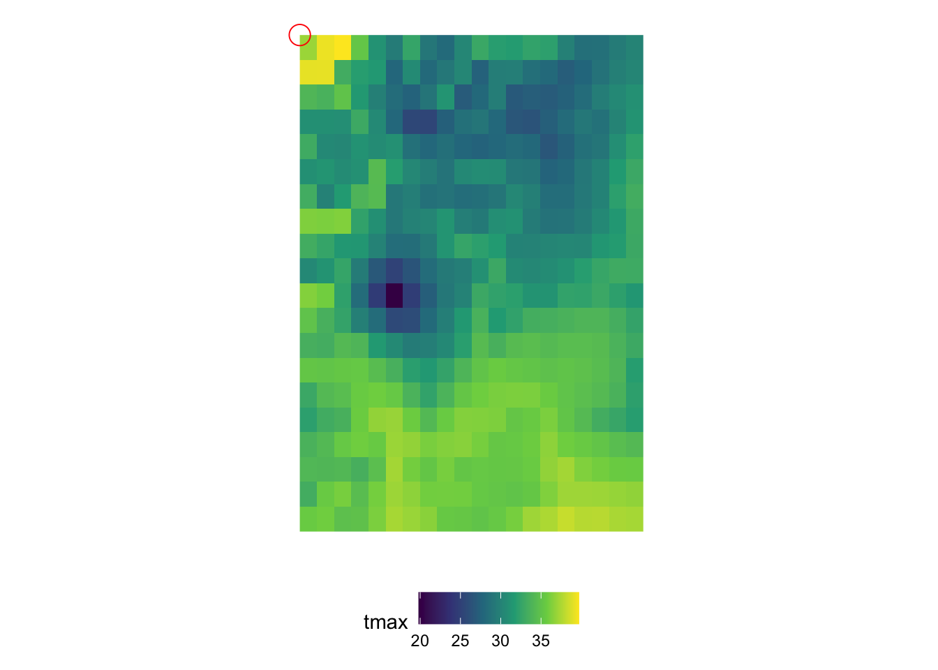
You can consider the 2D x-y surface as a matrix, where the location of a cell is defined by the row number and column number. Since the from for x is 1 and to for x is 20, we have 20 columns. Similarly, since the from for y is 1 and to for y is 20, we have 20 rows. The offset value of the x and y dimensions is the longitude and latitude of the upper-left corner point of the upper left cell of the 2D x-y surface, respectively (the red circle i@fig-two-d-map).2 As refsys indicates, they are in NAD83 GCS. The longitude of the upper-left corner point of all the cells in the \(j\)th column (from the left) of the 2D x-y surface is -121.7291667 + \((j-1)\times\) 0.0416667, where -121.7291667 is offset for x and 0.0416667 is delta for x. Similarly, the latitude of the upper-left corner point of all the cells in the \(i\)th row (from the top) of the 2D x-y surface is 46.6458333 +\((i-1)\times\) -0.0416667, where 46.6458333 is offset for y and -0.0416667 is delta for y.
2 This changes depending on the delta of x and y. If both of the delta for x and y are positive, then the offset value of the x and y dimensions are the longitude and latitude of the upper-left corner point of the lower-left cell of the 2D x-y surface.
The dimension characteristics of x and y are shared by all the layers across the date dimension, and a particular combination of x and y indexes refers to exactly the same location on the earth in all the layers across dates (of course). In the date dimension, we have 10 date values since the from for date is 1 and to for date is 10. The refsys of the date dimension is Date. Since the offset is 2009-08-11 and delta is 1, \(k\)th layer represents tmax values for August \(11+k-1\), 2009.
Putting all this information together, we have 20 by 20 x-y surfaces stacked over the date dimension (10 layers), thus making up a 20 by 20 by 10 three-dimensional array (or cube) as shown in the figure below (Figure 6.2).
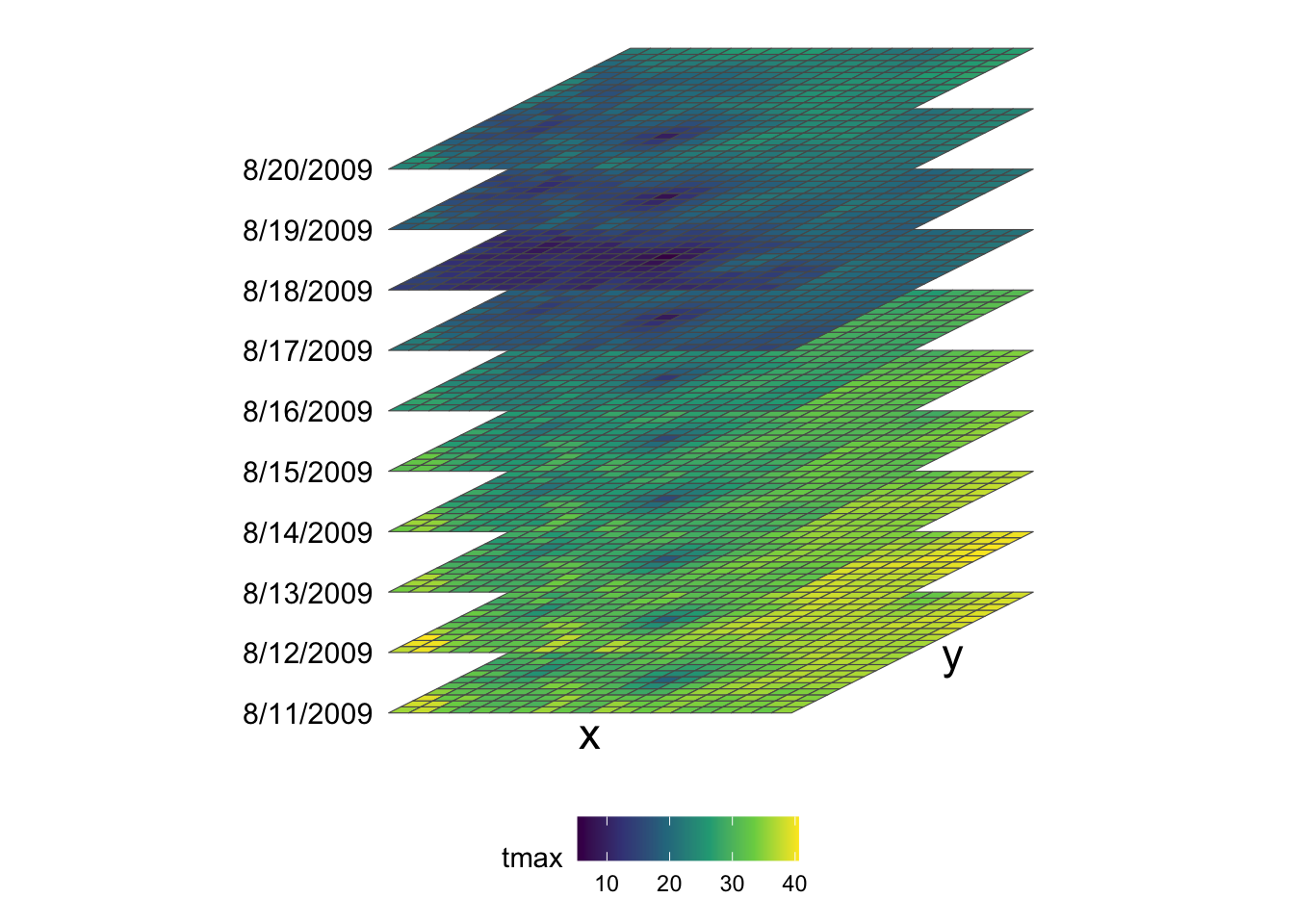
Remember that prcp_tmax_PRISM_m8_y09 also has another attribute (ppt) which is structured exactly the same way as tmax. So, prcp_tmax_PRISM_m8_y09 basically has four dimensions: attribute, x, y, and date.
It is not guaranteed that all the dimensions are regularly spaced or timed. For an irregular dimension, dimension values themselves are stored in values instead of using indexes, offset, and delta to find dimension values. For example, if you observe satellite data with 6-day gaps sometimes and 7-day gaps other times, then the date dimension would be irregular. We will see a made-up example of irregular time dimension in Section 6.5.
6.2 Some basic operations on stars objects
6.2.1 Create a new attribute and drop a attribute
You can add a new attribute to a stars object just like you add a variable to a data.frame.
#--- define a new variable which is tmax - 20 ---#
prcp_tmax_PRISM_m8_y09$tmax_less_20 <- prcp_tmax_PRISM_m8_y09$tmax - 20
As you can see below, prcp_tmax_PRISM_m8_y09 now has tmax_less_20 as an attribute.
prcp_tmax_PRISM_m8_y09stars object with 3 dimensions and 3 attributes
attribute(s):
Min. 1st Qu. Median Mean 3rd Qu. Max.
ppt 0.000 0.00000 0.000 1.292334 0.01100 30.851
tmax 1.833 17.55575 21.483 22.035435 26.54275 39.707
tmax_less_20 -18.167 -2.44425 1.483 2.035435 6.54275 19.707
dimension(s):
from to offset delta refsys point x/y
x 1 20 -121.7 0.04167 NAD83 FALSE [x]
y 1 20 46.65 -0.04167 NAD83 FALSE [y]
date 1 10 2009-08-11 1 days Date NA You can drop an attribute by assining NULL to the attribute you want to drop.
prcp_tmax_PRISM_m8_y09$tmax_less_20 <- NULL

prcp_tmax_PRISM_m8_y09
stars object with 3 dimensions and 2 attributes
attribute(s):
Min. 1st Qu. Median Mean 3rd Qu. Max.
ppt 0.000 0.00000 0.000 1.292334 0.01100 30.851
tmax 1.833 17.55575 21.483 22.035435 26.54275 39.707
dimension(s):
from to offset delta refsys point x/y
x 1 20 -121.7 0.04167 NAD83 FALSE [x]
y 1 20 46.65 -0.04167 NAD83 FALSE [y]
date 1 10 2009-08-11 1 days Date NA
6.2.2 Subset a stars object by index
In order to access the value of an attribute (say ppt) at a particular location at a particular time from the stars object (prcp_tmax_PRISM_m8_y09), you need to tell R that you are interested in the ppt attribute and specify the corresponding index of x, y, and date. Here, is how you get the ppt value of (3, 4) cell at date = 10.
prcp_tmax_PRISM_m8_y09["ppt", 3, 4, 10]stars object with 3 dimensions and 1 attribute
attribute(s):
Min. 1st Qu. Median Mean 3rd Qu. Max.
ppt 0 0 0 0 0 0
dimension(s):
from to offset delta refsys point x/y
x 3 3 -121.7 0.04167 NAD83 FALSE [x]
y 4 4 46.65 -0.04167 NAD83 FALSE [y]
date 10 10 2009-08-11 1 days Date NA This is very much similar to accessing a value from a matrix except that we have more dimensions. The first argument selects the attribute of interest, 2nd x, 3rd y, and 4th date.
Of course, you can subset a stars object to access the value of multiple cells like this:
prcp_tmax_PRISM_m8_y09["ppt", 3:6, 3:4, 5:10]stars object with 3 dimensions and 1 attribute
attribute(s):
Min. 1st Qu. Median Mean 3rd Qu. Max.
ppt 0 0 0 0.043125 0 0.546
dimension(s):
from to offset delta refsys point x/y
x 3 6 -121.7 0.04167 NAD83 FALSE [x]
y 3 4 46.65 -0.04167 NAD83 FALSE [y]
date 5 10 2009-08-11 1 days Date NA 6.2.3 Set attribute names
When you read a raster dataset from a GeoTIFF file, the attribute name is the file name by default. So, you will often encounter cases where you want to change the attribute name. You can set the name of attributes using setNames().
Note that the attribute names of prcp_tmax_PRISM_m8_y09 (original datar) have not changed after this operation (just like dplyr::mutate() or other dplyr functions do):
prcp_tmax_PRISM_m8_y09stars object with 3 dimensions and 2 attributes
attribute(s):
Min. 1st Qu. Median Mean 3rd Qu. Max.
ppt 0.000 0.00000 0.000 1.292334 0.01100 30.851
tmax 1.833 17.55575 21.483 22.035435 26.54275 39.707
dimension(s):
from to offset delta refsys point x/y
x 1 20 -121.7 0.04167 NAD83 FALSE [x]
y 1 20 46.65 -0.04167 NAD83 FALSE [y]
date 1 10 2009-08-11 1 days Date NA If you want to reflect changes in the variable names while keeping the same object name, you need to assign the output of setNames() to the object as follows:
We will be using this function in Section 6.7.2.
6.2.4 Get the coordinate reference system
You can get the CRS of a stars object using sf::st_crs(), which is actually the same function name that we used to extract the CRS of an sf object.
sf::st_crs(prcp_tmax_PRISM_m8_y09)Coordinate Reference System:
User input: NAD83
wkt:
GEOGCRS["NAD83",
DATUM["North American Datum 1983",
ELLIPSOID["GRS 1980",6378137,298.257222101004,
LENGTHUNIT["metre",1]]],
PRIMEM["Greenwich",0,
ANGLEUNIT["degree",0.0174532925199433]],
CS[ellipsoidal,2],
AXIS["geodetic latitude (Lat)",north,
ORDER[1],
ANGLEUNIT["degree",0.0174532925199433]],
AXIS["geodetic longitude (Lon)",east,
ORDER[2],
ANGLEUNIT["degree",0.0174532925199433]],
ID["EPSG",4269]]You will use this to change the projection of vector datasets when you interact them:
- crop the
starsraster dataset to the spatial extent ofsfobjects - extract values from the
starsraster dataset forsfobjects
as we will see in Chapter 5. Notice also that we used exactly the same function name (sf::st_crs()) to get the CRS of sf objects (see Chapter 2).
6.2.5 Get the dimension characteristics and values
You can access these dimension values using st_dimensions().
#--- get dimension characteristics ---#
(
  dim_prcp_tmin <- stars::st_dimensions(prcp_tmax_PRISM_m8_y09)
)
from to offset delta refsys point x/y
x 1 20 -121.7 0.04167 NAD83 FALSE [x]
y 1 20 46.65 -0.04167 NAD83 FALSE [y]
date 1 10 2009-08-11 1 days Date NA The following shows what we can get from this object.
str(dim_prcp_tmin)List of 3
$ x :List of 7
..$ from : num 1
..$ to : num 20
..$ offset: num -122
..$ delta : num 0.0417
..$ refsys:List of 2
.. ..$ input: chr "NAD83"
.. ..$ wkt : chr "GEOGCRS[\"NAD83\",\n DATUM[\"North American Datum 1983\",\n ELLIPSOID[\"GRS 1980\",6378137,298.257222"| __truncated__
.. ..- attr(*, "class")= chr "crs"
..$ point : logi FALSE
..$ values: NULL
..- attr(*, "class")= chr "dimension"
$ y :List of 7
..$ from : num 1
..$ to : num 20
..$ offset: num 46.6
..$ delta : num -0.0417
..$ refsys:List of 2
.. ..$ input: chr "NAD83"
.. ..$ wkt : chr "GEOGCRS[\"NAD83\",\n DATUM[\"North American Datum 1983\",\n ELLIPSOID[\"GRS 1980\",6378137,298.257222"| __truncated__
.. ..- attr(*, "class")= chr "crs"
..$ point : logi FALSE
..$ values: NULL
..- attr(*, "class")= chr "dimension"
$ date:List of 7
..$ from : num 1
..$ to : int 10
..$ offset: Date[1:1], format: "2009-08-11"
..$ delta : 'difftime' num 1
.. ..- attr(*, "units")= chr "days"
..$ refsys: chr "Date"
..$ point : logi NA
..$ values: NULL
..- attr(*, "class")= chr "dimension"
- attr(*, "raster")=List of 4
..$ affine : num [1:2] 0 0
..$ dimensions : chr [1:2] "x" "y"
..$ curvilinear: logi FALSE
..$ blocksizes : int [1:10, 1:2] 20 20 20 20 20 20 20 20 20 20 ...
.. ..- attr(*, "dimnames")=List of 2
.. .. ..$ : NULL
.. .. ..$ : chr [1:2] "x" "y"
..- attr(*, "class")= chr "stars_raster"
- attr(*, "class")= chr "dimensions"For example, you can get offset of x as follows:
dim_prcp_tmin$x$offset[1] -121.7292You can extract dimension values using stars::st_get_dimension_values(). For example, to get values of date,
#--- get date values ---#
stars::st_get_dimension_values(prcp_tmax_PRISM_m8_y09, "date") [1] "2009-08-11" "2009-08-12" "2009-08-13" "2009-08-14" "2009-08-15"
[6] "2009-08-16" "2009-08-17" "2009-08-18" "2009-08-19" "2009-08-20"This can be handy as you will see in Section 8.4.2. Later in Section 6.5, we will learn how to set dimensions using stars::st_set_dimensions().
6.2.6 Attributes to dimensions, and vice versa
You can make attributes to dimensions using base::merge().
(
prcp_tmax_four <- base::merge(prcp_tmax_PRISM_m8_y09)
)stars object with 4 dimensions and 1 attribute
attribute(s):
Min. 1st Qu. Median Mean 3rd Qu. Max.
ppt.tmax 0 0 11.799 11.66388 21.535 39.707
dimension(s):
from to offset delta refsys point values x/y
x 1 20 -121.7 0.04167 NAD83 FALSE NULL [x]
y 1 20 46.65 -0.04167 NAD83 FALSE NULL [y]
date 1 10 2009-08-11 1 days Date NA NULL
attributes 1 2 NA NA NA NA ppt , tmax As you can see, the new stars object has an additional dimension called attributes, which represents attributes and has two dimension values: the first for ppt and second for tmax. Now, if you want to access ppt, you can do the following:
prcp_tmax_four[, , , , "ppt"]stars object with 4 dimensions and 1 attribute
attribute(s):
Min. 1st Qu. Median Mean 3rd Qu. Max.
ppt.tmax 0 0 0 1.292334 0.011 30.851
dimension(s):
from to offset delta refsys point values x/y
x 1 20 -121.7 0.04167 NAD83 FALSE NULL [x]
y 1 20 46.65 -0.04167 NAD83 FALSE NULL [y]
date 1 10 2009-08-11 1 days Date NA NULL
attributes 1 1 NA NA NA NA ppt We can do this because the merge kept the attribute names as dimension values as you can see in values.
You can revert it back to the original state using base::split(). Since we want the fourth dimension to dissolve,
base::split(prcp_tmax_four, 4)stars object with 3 dimensions and 2 attributes
attribute(s):
Min. 1st Qu. Median Mean 3rd Qu. Max.
ppt 0.000 0.00000 0.000 1.292334 0.01100 30.851
tmax 1.833 17.55575 21.483 22.035435 26.54275 39.707
dimension(s):
     from to     offset    delta refsys point x/y
x       1 20     -121.7  0.04167  NAD83 FALSE [x]
y       1 20      46.65 -0.04167  NAD83 FALSE [y]
date 1 10 2009-08-11 1 days Date NA 6.3 Quick visualization for exploration
You can use plot() to have a quick static map and tmap::mapview() or the tmap package for interactive views.
plot(prcp_tmax_PRISM_m8_y09["tmax", , , ])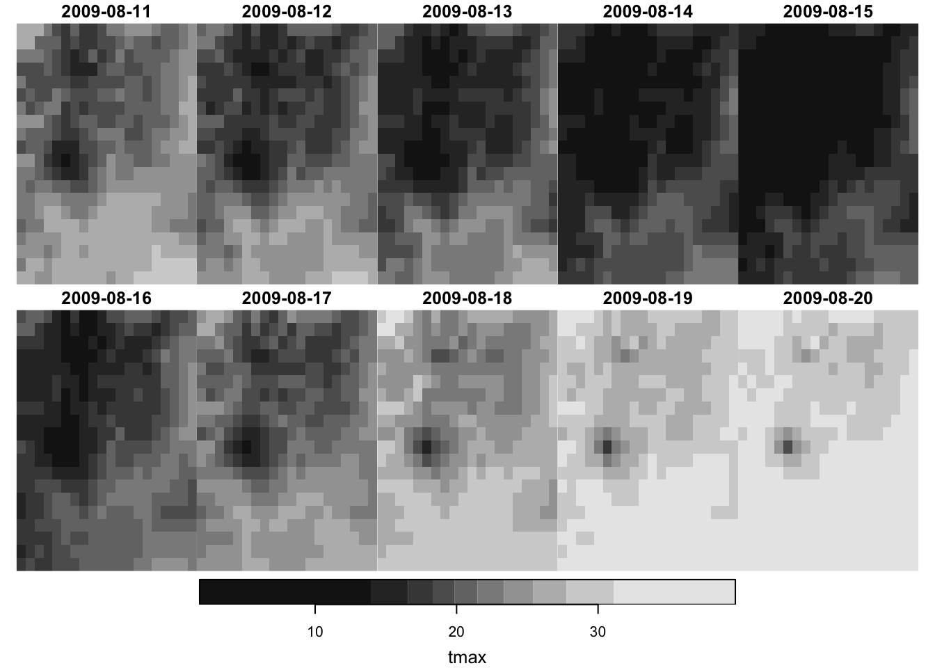
It only plots the first attribute if the stars object has multiple attributes:
plot(prcp_tmax_PRISM_m8_y09)
, which is identical with this:
plot(prcp_tmax_PRISM_m8_y09["ppt", , , ])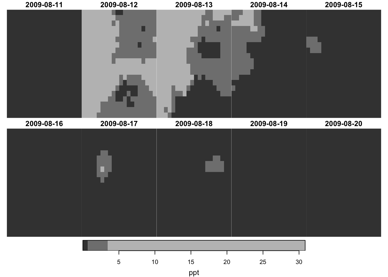
6.4 Reading and writing raster data
There are so many formats in which raster data is stored. Some of the common ones include GeoTIFF, netCDF, GRIB. All the available GDAL drivers for reading and writing raster data can be found by the following code:
sf::st_drivers(what = "raster") %>% DT::datatable()6.4.1 Reading raster data
You can use stars::read_stars() to read a raster data file. It is very unlikely that the raster file you are trying to read is not in one of the supported formats.
For example, you can read a GeoTIFF file as follows:
(
  ppt_m1_y09_stars <- stars::read_stars("Data/PRISM_ppt_y2009_m1.tif")
)
stars object with 3 dimensions and 1 attribute
attribute(s), summary of first 1e+05 cells:
Min. 1st Qu. Median Mean 3rd Qu. Max. NA's
PRISM_ppt_y2009_m1.tif 0 0 0.436 3.543222 3.4925 56.208 60401
dimension(s):
from to offset delta refsys point
x 1 1405 -125 0.04167 NAD83 FALSE
y 1 621 49.94 -0.04167 NAD83 FALSE
band 1 31 NA NA NA NA
values
x NULL
y NULL
band PRISM_ppt_stable_4kmD2_20090101_bil,...,PRISM_ppt_stable_4kmD2_20090131_bil
x/y
x [x]
y [y]
band This one imports a raw PRISM data stored as a BIL file.
(
  prism_tmax_20180701 <- stars::read_stars("Data/PRISM_tmax_stable_4kmD2_20180701_bil/PRISM_tmax_stable_4kmD2_20180701_bil.bil")
)
stars object with 2 dimensions and 1 attribute
attribute(s):
Min. 1st Qu. Median Mean 3rd Qu. Max.
PRISM_tmax_stable_4kmD2_201... 3.623 25.318 31.596 29.50749 33.735 48.008
NA's
PRISM_tmax_stable_4kmD2_201... 390874
dimension(s):
from to offset delta refsys x/y
x 1 1405 -125 0.04167 NAD83 [x]
y 1 621 49.94 -0.04167 NAD83 [y]You can import multiple raster data files into one stars object by simply supplying a vector of file names:
files <-
  c(
    "Data/PRISM_tmax_stable_4kmD2_20180701_bil/PRISM_tmax_stable_4kmD2_20180701_bil.bil",
    "Data/PRISM_tmax_stable_4kmD2_20180702_bil/PRISM_tmax_stable_4kmD2_20180702_bil.bil"
  )

(
  prism_tmax_201807_two <- stars::read_stars(files)
)
stars object with 2 dimensions and 2 attributes
attribute(s):
Min. 1st Qu. Median Mean 3rd Qu. Max.
1_bil/PRISM_tmax_stable_4km... 3.623 25.318 31.596 29.50749 33.735 48.008
2_bil/PRISM_tmax_stable_4km... 0.808 26.505 30.632 29.93235 33.632 47.999
NA's
1_bil/PRISM_tmax_stable_4km... 390874
2_bil/PRISM_tmax_stable_4km... 390874
dimension(s):
from to offset delta refsys x/y
x 1 1405 -125 0.04167 NAD83 [x]
y 1 621 49.94 -0.04167 NAD83 [y]As you can see, each file becomes an attribute. It is more convenient to have them as layers stacked along the third dimension. To do that you can add along = 3 option as follows:
(
  prism_tmax_201807_two <- stars::read_stars(files, along = 3)
)
stars object with 3 dimensions and 1 attribute
attribute(s), summary of first 1e+05 cells:
Min. 1st Qu. Median Mean 3rd Qu. Max.
PRISM_tmax_stable_4kmD2_201... 4.693 19.5925 23.653 22.05224 24.5945 33.396
NA's
PRISM_tmax_stable_4kmD2_201... 60401
dimension(s):
from to offset delta refsys
x 1 1405 -125 0.04167 NAD83
y 1 621 49.94 -0.04167 NAD83
new_dim 1 2 NA NA NA
values
x NULL
y NULL
new_dim 1_bil/PRISM_tmax_stable_4kmD2_20180701, 2_bil/PRISM_tmax_stable_4kmD2_20180702
x/y
x [x]
y [y]
new_dim Note that while the GeoTIFF format (and many other formats) can store multi-band (multi-layer) raster data allowing for an additional dimension beyond x and y, it does not store the values of the dimension like the date dimension we saw in prcp_tmax_PRISM_m8_y09. So, when you read a multi-layer raster data saved as a GeoTIFF, the third dimension of the resulting stars object will always be called band without any explicit time information. On the other hand, netCDF files are capable of storing the time dimension values. So, when you read a netCDF file with valid time dimension, you will have time dimension when it is read.
(
  stars::read_ncdf(system.file("nc/bcsd_obs_1999.nc", package = "stars"))
)
stars object with 3 dimensions and 2 attributes
attribute(s):
Min. 1st Qu. Median Mean 3rd Qu. Max. NA's
pr [mm/m] 0.5900000 56.139999 81.88000 101.26433 121.07250 848.54999 7116
tas [C] -0.4209678 8.898887 15.65763 15.48932 21.77979 29.38581 7116
dimension(s):
from to offset delta refsys values x/y
longitude 1 81 -85 0.125 WGS 84 NULL [x]
latitude 1 33 33 0.125 WGS 84 NULL [y]
time 1 12 NA NA POSIXct 1999-01-31,...,1999-12-31 The refsys of the time dimension is POSIXct, which is one of the date classes.
6.4.2 Writing a stars object to a file
You can write a stars object to a file using stars::write_stars() using one of the GDAL drivers.
Let’s save prcp_tmax_PRISM_m8_y09["tmax",,,], which has date dimension whose refsys is Date.
stars::write_stars(prcp_tmax_PRISM_m8_y09["tmax", , , ], "Data/tmax_m8_y09_from_stars.tif")Let’s read the file we just saved.
stars::read_stars("Data/tmax_m8_y09_from_stars.tif")stars object with 3 dimensions and 1 attribute
attribute(s):
Min. 1st Qu. Median Mean 3rd Qu. Max.
tmax_m8_y09_from_stars.tif 1.833 17.55575 21.483 22.03543 26.54275 39.707
dimension(s):
from to offset delta refsys point x/y
x 1 20 -121.7 0.04167 NAD83 FALSE [x]
y 1 20 46.65 -0.04167 NAD83 FALSE [y]
band 1 10 NA NA NA NA Notice that the third dimension is now called band and all the date information is lost. The loss of information happened when we saved prcp_tmax_PRISM_m8_y09["tmax",,,] as a GeoTIFF file. One easy way to avoid this problem is to just save a stars object as an R dataset.
#--- save it as an rds file ---#
saveRDS(prcp_tmax_PRISM_m8_y09["tmax", , , ], "Data/tmax_m8_y09_from_stars.rds")
#--- read it back ---#
readRDS("Data/tmax_m8_y09_from_stars.rds")stars object with 3 dimensions and 1 attribute
attribute(s):
Min. 1st Qu. Median Mean 3rd Qu. Max.
tmax 1.833 17.55575 21.483 22.03543 26.54275 39.707
dimension(s):
from to offset delta refsys point x/y
x 1 20 -121.7 0.04167 NAD83 FALSE [x]
y 1 20 46.65 -0.04167 NAD83 FALSE [y]
date 1 10 2009-08-11 1 days Date NA As you can see, date information is retained. So, if you are the only one who uses this data or all of your team members use R, then this is a nice solution to the problem. At the moment, it is not possible to use stars::write_stars() to write to a netCDF file that supports the third dimension as time. However, this may not be the case for a long time (See the discussion here).
6.5 Setting the time dimension manually
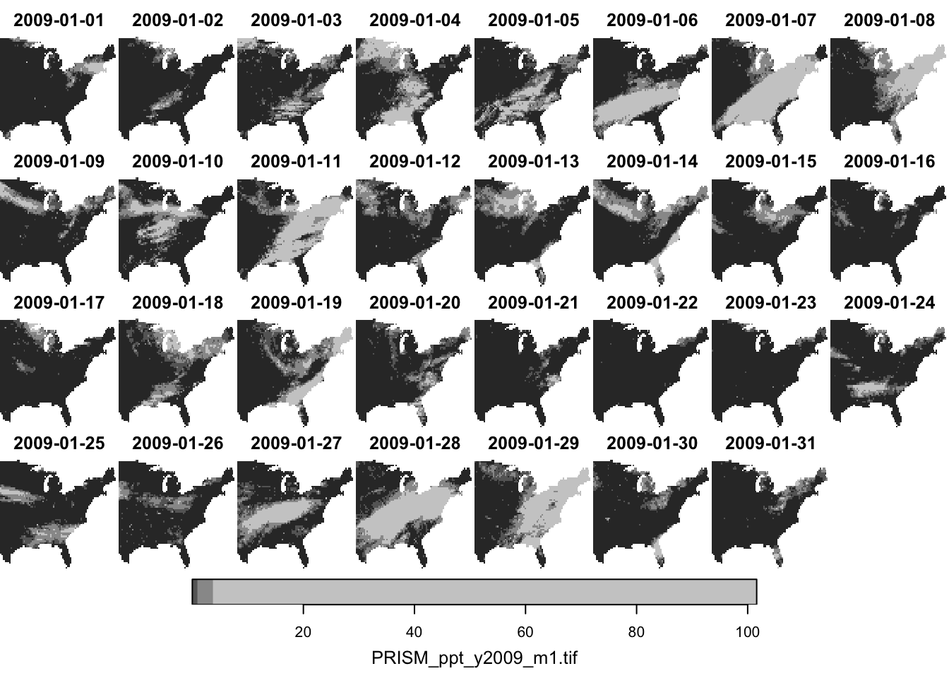
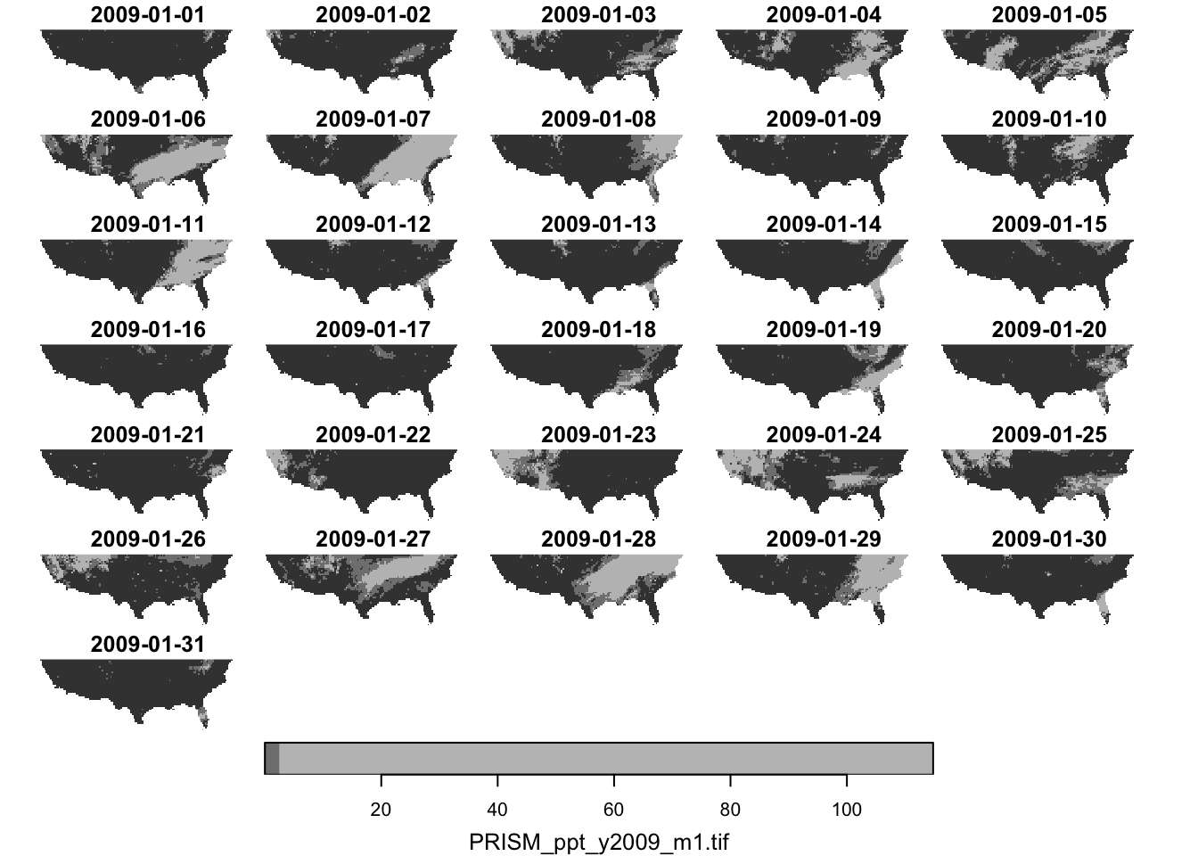
For this section, we will use PRISM precipitation data for U.S. for January, 2009.
(
  ppt_m1_y09_stars <- stars::read_stars("Data/PRISM_ppt_y2009_m1.tif")
)
stars object with 3 dimensions and 1 attribute
attribute(s), summary of first 1e+05 cells:
Min. 1st Qu. Median Mean 3rd Qu. Max. NA's
PRISM_ppt_y2009_m1.tif 0 0 0.436 3.543222 3.4925 56.208 60401
dimension(s):
from to offset delta refsys point
x 1 1405 -125 0.04167 NAD83 FALSE
y 1 621 49.94 -0.04167 NAD83 FALSE
band 1 31 NA NA NA NA
values
x NULL
y NULL
band PRISM_ppt_stable_4kmD2_20090101_bil,...,PRISM_ppt_stable_4kmD2_20090131_bil
x/y
x [x]
y [y]
band As you can see, when you read a GeoTIFF file, the third dimension will always be called band because GeoTIFF format does not support dimension values for the third dimension.3
3 In Section 6.1, we read an rds, which is a stars object with dimension name set manually.
You can use st_set_dimension() to set the third dimension (called band) as the time dimension using Date object. This can be convenient when you would like to filter the data by date using filter() as we will see later.
For ppt_m1_y09_stars, precipitation is observed on a daily basis from January 1, 2009 to January 31, 2009, where the band value of x corresponds to January x, 2009. So, we can first create a vector of dates as follows (If you are not familiar with Dates and the lubridate pacakge, this is a good resource to learn them.):
#--- starting date ---#
start_date <- lubridate::ymd("2009-01-01")

#--- ending date ---#
end_date <- lubridate::ymd("2009-01-31")

#--- sequence of dates  ---#
(
dates_ls_m1 <- seq(start_date, end_date, "days")
)
[1] "2009-01-01" "2009-01-02" "2009-01-03" "2009-01-04" "2009-01-05"
[6] "2009-01-06" "2009-01-07" "2009-01-08" "2009-01-09" "2009-01-10"
[11] "2009-01-11" "2009-01-12" "2009-01-13" "2009-01-14" "2009-01-15"
[16] "2009-01-16" "2009-01-17" "2009-01-18" "2009-01-19" "2009-01-20"
[21] "2009-01-21" "2009-01-22" "2009-01-23" "2009-01-24" "2009-01-25"
[26] "2009-01-26" "2009-01-27" "2009-01-28" "2009-01-29" "2009-01-30"
[31] "2009-01-31"We can then use stars::st_set_dimensions() to change the third dimension to the dimension of date.
stars::st_set_dimensions(
  stars object,
  dimension,
  values = dimension values,
  names = name of the dimension
 )
(
ppt_m1_y09_stars <-
stars::st_set_dimensions(
ppt_m1_y09_stars,
3,
values = dates_ls_m1,
names = "date"
)
)stars object with 3 dimensions and 1 attribute
attribute(s), summary of first 1e+05 cells:
Min. 1st Qu. Median Mean 3rd Qu. Max. NA's
PRISM_ppt_y2009_m1.tif 0 0 0.436 3.543222 3.4925 56.208 60401
dimension(s):
from to offset delta refsys point x/y
x 1 1405 -125 0.04167 NAD83 FALSE [x]
y 1 621 49.94 -0.04167 NAD83 FALSE [y]
date 1 31 2009-01-01 1 days Date NA As you can see, the third dimension has become date. The value of offset for the date dimension has become 2009-01-01 meaning the starting date value is now 2009-01-01. Further, the value of delta is now 1 days, so date dimension of x corresponds to 2009-01-01 + x - 1 = 2009-01-x.
Note that the date dimension does not have to be regularly spaced. For example, you may have satellite images available for your area with a 5-day interval sometimes and a 6-day interval other times. This is perfectly fine. As an illustration, I will create a wrong sequence of dates for this data with a 2-day gap in the middle and assign them to the date dimension to see what happens.
#--- 2009-01-23 removed and 2009-02-01 added ---#
(
  dates_ls_wrong <- c(seq(start_date, end_date, "days")[-23], lubridate::ymd("2009-02-01"))
)
[1] "2009-01-01" "2009-01-02" "2009-01-03" "2009-01-04" "2009-01-05"
[6] "2009-01-06" "2009-01-07" "2009-01-08" "2009-01-09" "2009-01-10"
[11] "2009-01-11" "2009-01-12" "2009-01-13" "2009-01-14" "2009-01-15"
[16] "2009-01-16" "2009-01-17" "2009-01-18" "2009-01-19" "2009-01-20"
[21] "2009-01-21" "2009-01-22" "2009-01-24" "2009-01-25" "2009-01-26"
[26] "2009-01-27" "2009-01-28" "2009-01-29" "2009-01-30" "2009-01-31"
[31] "2009-02-01"Now assign these date values to ppt_m1_y09_stars:
#--- set date values ---#
(
  ppt_m1_y09_stars_wrong <-
    stars::st_set_dimensions(
      ppt_m1_y09_stars,
      3,
      values = dates_ls_wrong,
      names = "date"
    )
)
stars object with 3 dimensions and 1 attribute
attribute(s), summary of first 1e+05 cells:
Min. 1st Qu. Median Mean 3rd Qu. Max. NA's
PRISM_ppt_y2009_m1.tif 0 0 0.436 3.543222 3.4925 56.208 60401
dimension(s):
from to offset delta refsys point values x/y
x 1 1405 -125 0.04167 NAD83 FALSE NULL [x]
y 1 621 49.94 -0.04167 NAD83 FALSE NULL [y]
date 1 31 NA NA Date NA 2009-01-01,...,2009-02-01 Since the step between the date values is no longer \(1\) day for the entire sequence, the value of delta is now NA. However, notice that the value of date is no longer NULL. Since the date is not regular, you cannot represent date using three values (from, to, and delta) any more, and date values for each observation have to be stored now.
Finally, note that just applying stars::st_set_dimensions() to a stars object does not change the dimension of the stars object (just like setNames() as we discussed above).
ppt_m1_y09_starsstars object with 3 dimensions and 1 attribute
attribute(s), summary of first 1e+05 cells:
Min. 1st Qu. Median Mean 3rd Qu. Max. NA's
PRISM_ppt_y2009_m1.tif 0 0 0.436 3.543222 3.4925 56.208 60401
dimension(s):
from to offset delta refsys point x/y
x 1 1405 -125 0.04167 NAD83 FALSE [x]
y 1 621 49.94 -0.04167 NAD83 FALSE [y]
date 1 31 2009-01-01 1 days Date NA As you can see, the date dimension has not been altered. You need to assign the results of stars::st_set_dimensions() to a stars object to see the changes in the dimension reflected just like we did above with the right date values.
6.6 dplyr-like operations
You can use the dplyr language to do basic data operations on stars objects.
6.6.1 dplyr::filter()
The dplyr::filter() function allows you to subset data by dimension values: x, y, and band (here date).
spatial filtering
temporal filtering
Finally, since the date dimension is in Date, you can use Date math to filter the data.4
4 This is possible only because we have assigned date values to the band dimension above.
#--- dates after 2009-01-15  ---#
dplyr::filter(ppt_m1_y09_stars, date > lubridate::ymd("2009-01-21")) %>% plot()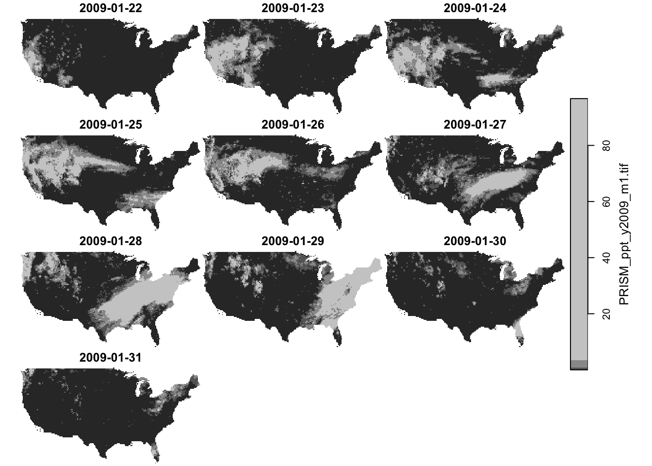
filter by attribute?
In case you are wondering, filtering by attribute is not possible. This makes sense, as doing so would disrupt the regular grid structure of raster data.
dplyr::filter(ppt_m1_y09_stars, ppt > 20)Error in `map2_int()`:
ℹ In index: 1.
Caused by error in `glubort()`:
! ``~``, `ppt > 20` must refer to exactly one dimension, not ``
6.6.2 dplyr::select()
The dply::select() function lets you pick certain attributes.
dplyr::select(prcp_tmax_PRISM_m8_y09, ppt)stars object with 3 dimensions and 1 attribute
attribute(s):
Min. 1st Qu. Median Mean 3rd Qu. Max.
ppt 0 0 0 1.292334 0.011 30.851
dimension(s):
from to offset delta refsys point x/y
x 1 20 -121.7 0.04167 NAD83 FALSE [x]
y 1 20 46.65 -0.04167 NAD83 FALSE [y]
date 1 10 2009-08-11 1 days Date NA
6.6.3 dplyr::mutate()
You can mutate attributes using the dplyr::mutate() function. For example, this can be useful to calculate NDVI in a stars object that has Red and NIR (spectral reflectance measurements in the red and near-infrared regions) as attributes. Here, we just simply convert the unit of precipitation from mm to inches.
#--- mm to inches ---#
dplyr::mutate(prcp_tmax_PRISM_m8_y09, ppt = ppt * 0.0393701)
stars object with 3 dimensions and 2 attributes
attribute(s):
Min. 1st Qu. Median Mean 3rd Qu. Max.
ppt 0.000 0.00000 0.000 0.0508793 4.330711e-04 1.214607
tmax 1.833 17.55575 21.483 22.0354348 2.654275e+01 39.707001
dimension(s):
from to offset delta refsys point x/y
x 1 20 -121.7 0.04167 NAD83 FALSE [x]
y 1 20 46.65 -0.04167 NAD83 FALSE [y]
date 1 10 2009-08-11 1 days Date NA
6.6.4 dplyr::pull()
You can extract attribute values using dplyr::pull().
#--- tmax values of the 1st date layer ---#
dplyr::pull(prcp_tmax_PRISM_m8_y09["tmax", , , 1], "tmax")
, , 1
[,1] [,2] [,3] [,4] [,5] [,6] [,7] [,8] [,9] [,10]
[1,] 25.495 27.150 22.281 19.553 21.502 19.616 21.664 24.458 21.712 19.326
[2,] 27.261 27.042 21.876 19.558 19.141 19.992 18.694 24.310 21.094 20.032
[3,] 27.568 21.452 23.220 19.428 18.974 19.366 20.293 24.418 20.190 21.127
[4,] 23.310 20.357 20.111 21.380 19.824 19.638 22.135 20.885 20.121 18.396
[5,] 19.571 20.025 18.407 19.142 19.314 22.759 22.652 19.566 18.817 16.065
[6,] 17.963 16.581 17.121 16.716 19.680 20.521 17.991 18.007 17.430 14.586
[7,] 20.911 19.202 16.309 14.496 17.429 19.083 18.509 18.723 17.645 16.415
[8,] 17.665 16.730 17.691 14.370 16.849 18.413 17.787 20.000 19.319 18.401
[9,] 16.795 18.091 20.460 16.405 18.331 19.005 19.142 21.226 21.184 19.520
[10,] 19.208 19.624 17.210 19.499 18.492 20.854 18.684 19.811 22.058 19.923
[11,] 23.148 18.339 19.676 20.674 18.545 21.126 19.013 19.722 21.843 21.271
[12,] 23.254 21.279 21.921 19.894 19.445 21.499 19.765 20.742 21.560 22.989
[13,] 23.450 21.956 19.813 18.970 20.173 20.567 21.152 20.932 19.836 20.347
[14,] 24.075 21.120 20.166 19.177 20.428 20.908 21.060 19.832 19.764 19.981
[15,] 24.318 20.943 20.024 20.022 19.040 19.773 20.452 20.152 20.321 20.304
[16,] 22.538 19.461 20.100 21.149 19.958 20.486 20.535 20.445 21.564 21.493
[17,] 20.827 20.192 21.165 22.369 21.488 22.031 21.552 21.089 21.687 23.375
[18,] 21.089 21.451 22.692 21.793 22.160 23.049 22.562 22.738 23.634 24.697
[19,] 22.285 22.992 23.738 23.497 24.255 25.177 25.411 24.324 24.588 26.032
[20,] 23.478 23.584 24.589 24.719 26.114 26.777 27.310 26.643 26.516 26.615
[,11] [,12] [,13] [,14] [,15] [,16] [,17] [,18] [,19] [,20]
[1,] 24.845 23.211 21.621 23.180 21.618 21.322 22.956 23.749 23.162 25.746
[2,] 24.212 21.820 21.305 22.960 22.806 22.235 23.604 23.689 25.597 25.933
[3,] 20.879 20.951 22.280 23.536 23.455 22.537 24.760 23.587 26.170 24.764
[4,] 17.435 18.681 22.224 24.122 25.828 25.604 25.298 22.817 24.438 24.835
[5,] 14.186 17.789 20.624 23.416 26.059 27.571 25.158 24.201 26.001 26.235
[6,] 10.188 15.632 19.907 22.660 25.268 27.469 27.376 27.488 27.278 27.558
[7,] 14.797 15.933 19.204 21.641 23.107 25.626 26.990 25.838 26.906 27.247
[8,] 17.325 18.299 19.691 21.553 21.840 23.754 26.099 25.270 26.282 26.981
[9,] 19.322 19.855 20.489 22.597 23.614 25.873 26.906 26.368 26.332 25.844
[10,] 20.241 21.800 22.111 24.128 25.765 27.105 27.200 25.491 26.306 25.663
[11,] 23.398 24.090 24.884 25.596 26.545 27.014 26.464 25.708 25.742 25.336
[12,] 22.576 21.996 23.874 26.447 26.955 26.871 25.533 25.576 25.610 25.902
[13,] 22.023 22.358 24.996 26.185 27.249 25.617 25.623 25.600 25.433 26.681
[14,] 20.974 23.533 25.388 25.975 27.316 26.199 26.090 25.920 25.767 27.956
[15,] 20.982 23.632 24.703 25.539 26.515 27.133 27.407 27.518 27.149 28.506
[16,] 22.500 24.012 25.282 25.751 25.212 25.290 26.058 28.258 28.290 29.842
[17,] 23.024 24.381 25.157 25.259 24.829 24.183 25.632 26.947 28.601 29.589
[18,] 24.016 24.425 24.965 24.930 24.482 23.274 25.412 26.733 28.494 29.656
[19,] 24.065 24.105 24.145 24.318 23.912 22.782 25.039 26.554 28.184 29.012
[20,] 23.979 24.321 23.477 22.135 22.395 22.189 24.944 26.542 27.923 28.849
6.7 Merging stars objects using c() and stars::st_mosaic()
6.7.1 Merging stars objects along the third dimension (band)
Here we learn how to merge multiple stars objects that have
- the same attributes
- the same spatial extent and resolution
- different bands (dates here)
For example, consider merging PRISM precipitation data in January and February. Both of them have exactly the same spatial extent and resolutions and represent the same attribute (precipitation). However, they differ in the third dimension (date). So, you are trying to stack data of the same attributes along the third dimension (date) while making sure that spatial correspondence is maintained. This merge is kind of like rbind() that stacks multiple data.frames vertically while making sure the variables are aligned correctly.
Let’s import the PRISM precipitation data for February, 2009.
#--- read the February ppt data ---#
(
  ppt_m2_y09_stars <- stars::read_stars("Data/PRISM_ppt_y2009_m2.tif")
)
stars object with 3 dimensions and 1 attribute
attribute(s), summary of first 1e+05 cells:
Min. 1st Qu. Median Mean 3rd Qu. Max. NA's
PRISM_ppt_y2009_m2.tif 0 0 0 0.1855858 0 11.634 60401
dimension(s):
from to offset delta refsys point
x 1 1405 -125 0.04167 NAD83 FALSE
y 1 621 49.94 -0.04167 NAD83 FALSE
band 1 28 NA NA NA NA
values
x NULL
y NULL
band PRISM_ppt_stable_4kmD2_20090201_bil,...,PRISM_ppt_stable_4kmD2_20090228_bil
x/y
x [x]
y [y]
band Note here that the third dimension of ppt_m2_y09_stars has not been changed to date.
Now, let’s try to merge the two:
#--- combine the two ---#
(
  ppt_m1_to_m2_y09_stars <- c(ppt_m1_y09_stars, ppt_m2_y09_stars, along = 3)
)
stars object with 3 dimensions and 1 attribute
attribute(s), summary of first 1e+05 cells:
Min. 1st Qu. Median Mean 3rd Qu. Max. NA's
PRISM_ppt_y2009_m1.tif 0 0 0.436 3.543222 3.4925 56.208 60401
dimension(s):
from to offset delta refsys point x/y
x 1 1405 -125 0.04167 NAD83 FALSE [x]
y 1 621 49.94 -0.04167 NAD83 FALSE [y]
date 1 59 2009-01-01 1 days Date NA As you noticed, the second object (ppt_m2_y09_stars) was assumed to have the same date characteristics as the first one: the data in February is observed daily (delta is 1 day). This causes no problem in this instance as the February data is indeed observed daily starting from 2009-02-01. However, be careful if you are appending the data that does not start from 1 day after (or more generally delta for the time dimension) the first data or the data that does not follow the same observation interval.
For this reason, it is advisable to first set the date values if it has not been set. Pretend that the February data actually starts from 2009-02-02 to 2009-03-01 to see what happens when the regular interval (delta) is not kept after merging.
#--- starting date ---#
start_date <- lubridate::ymd("2009-02-01")

#--- ending date ---#
end_date <- lubridate::ymd("2009-02-28")

#--- sequence of dates  ---#
dates_ls <- seq(start_date, end_date, "days")

#--- pretend the data actually starts from `2009-02-02` to `2009-03-01` ---#
(
  ppt_m2_y09_stars <-
    stars::st_set_dimensions(
      ppt_m2_y09_stars,
      3,
      values = c(dates_ls[-1], lubridate::ymd("2009-03-01")),
      name = "date"
    )
)
stars object with 3 dimensions and 1 attribute
attribute(s), summary of first 1e+05 cells:
Min. 1st Qu. Median Mean 3rd Qu. Max. NA's
PRISM_ppt_y2009_m2.tif 0 0 0 0.1855858 0 11.634 60401
dimension(s):
from to offset delta refsys point x/y
x 1 1405 -125 0.04167 NAD83 FALSE [x]
y 1 621 49.94 -0.04167 NAD83 FALSE [y]
date 1 28 2009-02-02 1 days Date NA If you merge the two,
c(ppt_m1_y09_stars, ppt_m2_y09_stars, along = 3)stars object with 3 dimensions and 1 attribute
attribute(s), summary of first 1e+05 cells:
Min. 1st Qu. Median Mean 3rd Qu. Max. NA's
PRISM_ppt_y2009_m1.tif 0 0 0.436 3.543222 3.4925 56.208 60401
dimension(s):
from to offset delta refsys point values x/y
x 1 1405 -125 0.04167 NAD83 FALSE NULL [x]
y 1 621 49.94 -0.04167 NAD83 FALSE NULL [y]
date 1 59 NA NA Date NA 2009-01-01,...,2009-03-01 The date dimension does not have delta any more, and correctly so because there is a one-day gap between the end date of the first stars object ("2009-01-31") and the start date of the second stars object ("2009-02-02"). So, all the date values are now stored in values.
6.7.2 Merging stars objects of different attributes
Here we learn how to merge multiple stars objects that have
- different attributes
- the same spatial extent and resolution
- the same bands (dates here)
For example, consider merging PRISM precipitation and tmax data in January. Both of them have exactly the same spatial extent and resolutions and the date characteristics (starting and ending on the same dates with the same time interval). However, they differ in what they represent: precipitation and tmax. This merge is kind of like cbind() that combines multiple data.frames of different variables while making sure the observation correspondence is correct.
Let’s read the daily tmax data for January, 2009:
(
  tmax_m8_y09_stars <-
    stars::read_stars("Data/PRISM_tmax_y2009_m1.tif") %>%
    #--- change the attribute name ---#
    setNames("tmax")
)
stars object with 3 dimensions and 1 attribute
attribute(s), summary of first 1e+05 cells:
Min. 1st Qu. Median Mean 3rd Qu. Max. NA's
tmax -17.898 -7.761 -2.248 -3.062721 1.718 7.994 60401
dimension(s):
from to offset delta refsys point
x 1 1405 -125 0.04167 NAD83 FALSE
y 1 621 49.94 -0.04167 NAD83 FALSE
band 1 31 NA NA NA NA
values
x NULL
y NULL
band PRISM_tmax_stable_4kmD2_20090101_bil,...,PRISM_tmax_stable_4kmD2_20090131_bil
x/y
x [x]
y [y]
band Now, let’s merge the PRISM ppt and tmax data in January, 2009.
c(ppt_m1_y09_stars, tmax_m8_y09_stars)Error in c.stars(ppt_m1_y09_stars, tmax_m8_y09_stars): don't know how to merge arrays: please specify parameter alongOops. Well, the problem is that the third dimension of the two objects is not the same. Even though we know that the xth element of their third dimension represent the same thing, they look different to R’s eyes. So, we first need to change the third dimension of tmax_m8_y09_stars to be consistent with the third dimension of ppt_m1_y09_stars (dates_ls_m1 was defined in Section 6.5).
(
  tmax_m8_y09_stars <- stars::st_set_dimensions(tmax_m8_y09_stars, 3, values = dates_ls_m1, names = "date")
)
stars object with 3 dimensions and 1 attribute
attribute(s), summary of first 1e+05 cells:
Min. 1st Qu. Median Mean 3rd Qu. Max. NA's
tmax -17.898 -7.761 -2.248 -3.062721 1.718 7.994 60401
dimension(s):
from to offset delta refsys point x/y
x 1 1405 -125 0.04167 NAD83 FALSE [x]
y 1 621 49.94 -0.04167 NAD83 FALSE [y]
date 1 31 2009-01-01 1 days Date NA Now, we can merge the two.
(
  ppt_tmax_m8_y09_stars <- c(ppt_m1_y09_stars, tmax_m8_y09_stars)
)
stars object with 3 dimensions and 2 attributes
attribute(s), summary of first 1e+05 cells:
Min. 1st Qu. Median Mean 3rd Qu. Max. NA's
PRISM_ppt_y2009_m1.tif 0.000 0.000 0.436 3.543222 3.4925 56.208 60401
tmax -17.898 -7.761 -2.248 -3.062721 1.7180 7.994 60401
dimension(s):
from to offset delta refsys point x/y
x 1 1405 -125 0.04167 NAD83 FALSE [x]
y 1 621 49.94 -0.04167 NAD83 FALSE [y]
date 1 31 2009-01-01 1 days Date NA As you can see, now we have another attribute called tmax.
6.7.3 Merging stars objects of different spatial extents
Here we learn how to merge multiple stars objects that have
- the same attributes
- different spatial extent but same resolution5
- the same bands (dates here)
5 Technically, you can actually merge stars objects of different spatial resolutions. But, you probably should not.
Some times you have multiple separate raster datasets that have different spatial coverages and would like to combine them into one. You can do that using stars::st_mosaic().
Let’s split tmax_m8_y09_stars into two parts (Figure 6.3 shows what they look like (only Jan 1, 1980)):
Code
Let’s combine the two using stars::st_mosaic():
tmax_combined <- stars::st_mosaic(tmax_1, tmax_2)Figure 6.4 shows what the combined object looks like.
Code
ggplot() +
  geom_stars(data = tmax_combined[, , , 1]) +
  theme_for_map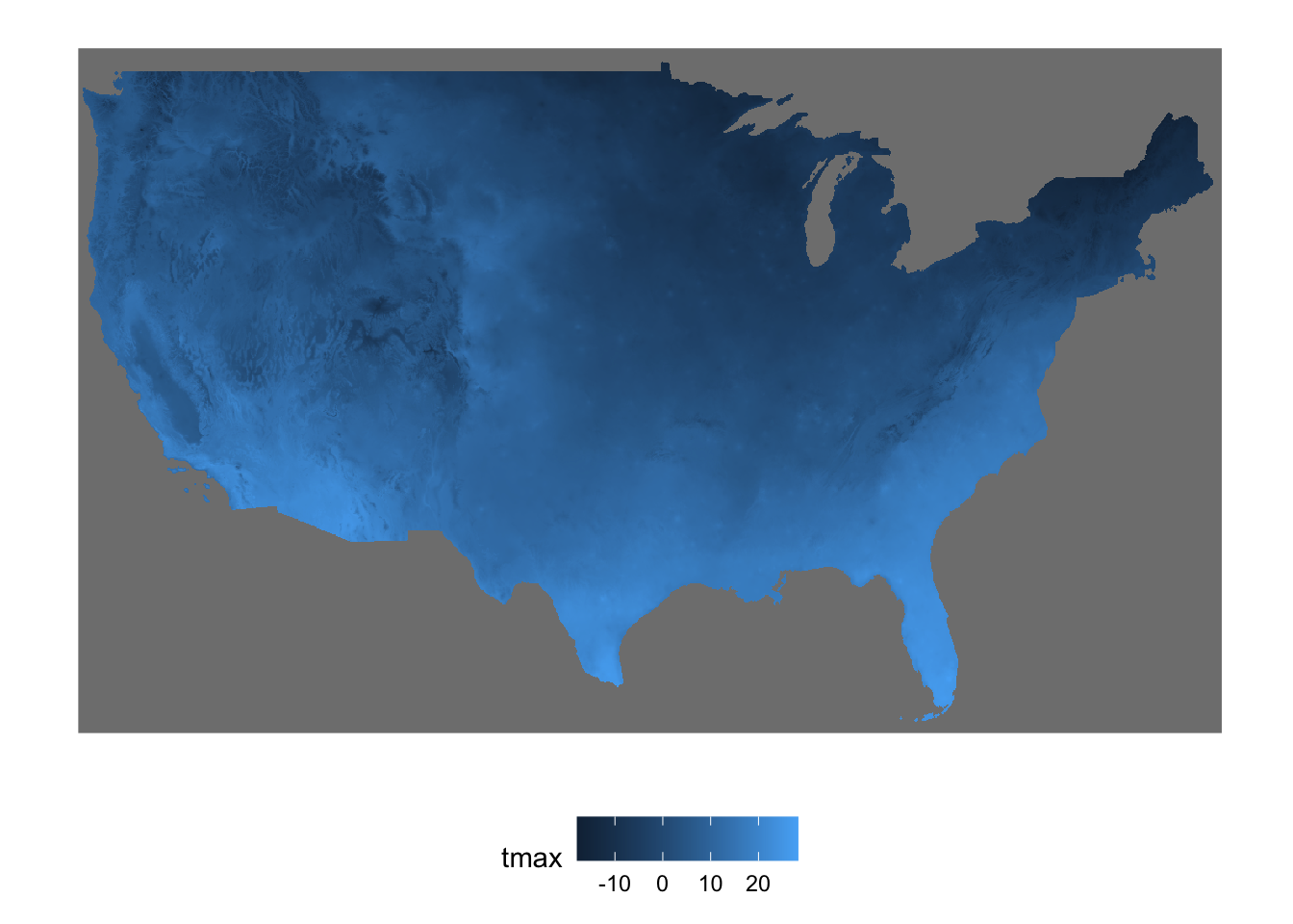
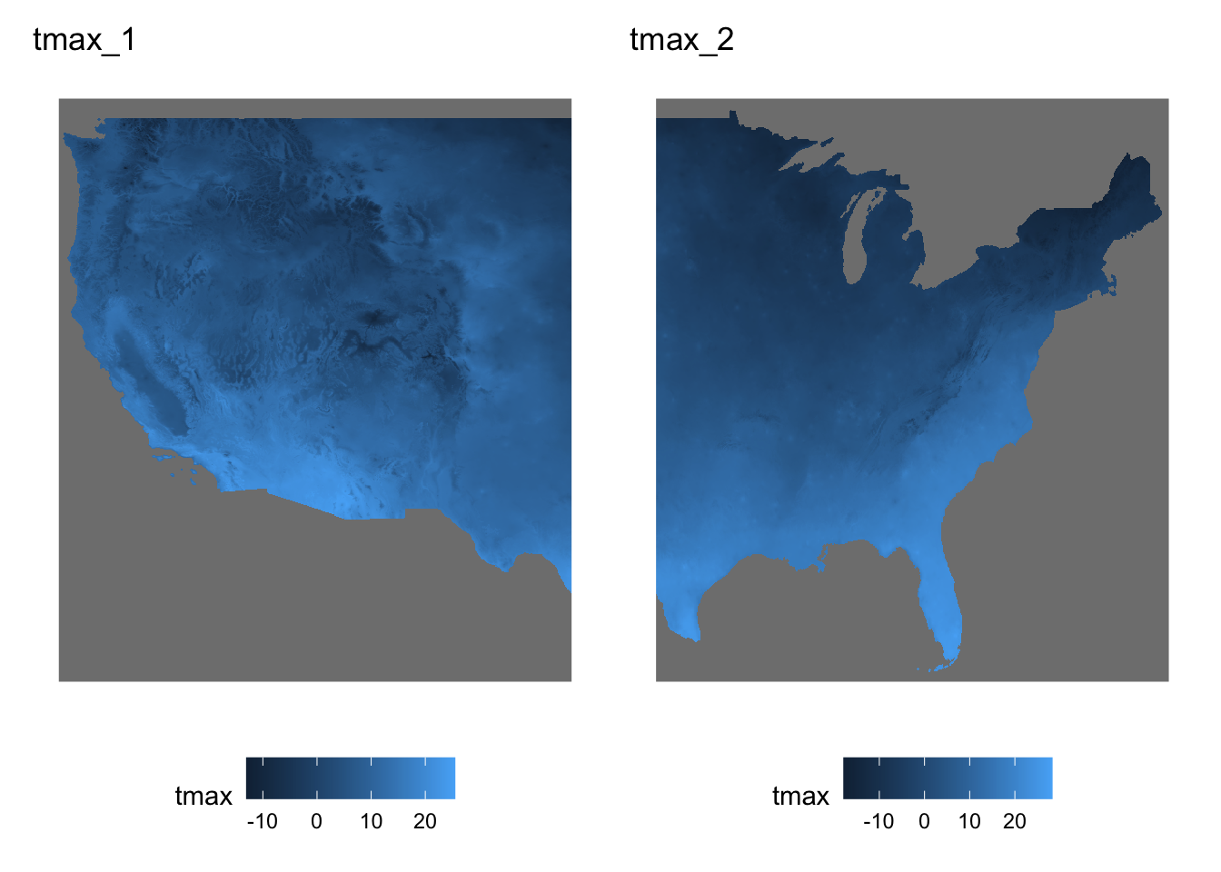
It is okay to have the two stars objects to be combined have a spatial overlap. The following split creates two stars objects with a spatial overlap (Figure 6.5 shows what they look like).
Code
g_1 <-
  ggplot() +
  geom_stars(data = tmax_m8_y09_stars[, , , 1], fill = NA) +
  geom_stars(data = tmax_1[, , , 1]) +
  theme_for_map +
  ggtitle("tmax_1")

g_2 <-
  ggplot() +
  geom_stars(data = tmax_m8_y09_stars[, , , 1], fill = NA) +
  geom_stars(data = tmax_2[, , , 1]) +
  theme_for_map +
  ggtitle("tmax_2")

library(patchwork)
g_1 / g_2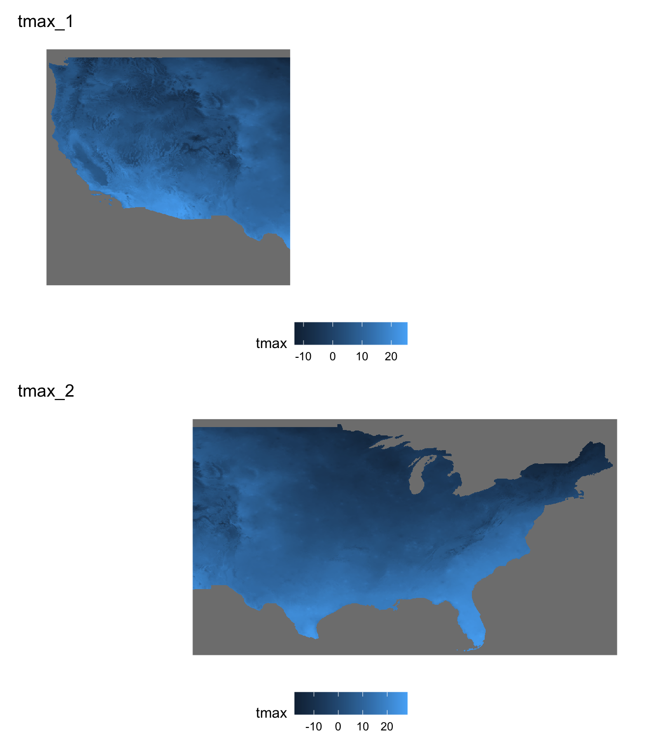
As you can see below, stars::st_mosaic() reconciles the spatial overlap between the two stars objects (Figure 6.6).
(
  tmax_combined <- stars::st_mosaic(tmax_1, tmax_2)
)
stars object with 3 dimensions and 1 attribute
attribute(s), summary of first 1e+05 cells:
Min. 1st Qu. Median Mean 3rd Qu. Max. NA's
tmax -17.898 -7.761 -2.248 -3.062721 1.718 7.994 60401
dimension(s):
from to offset delta refsys x/y
x 1 1405 -125 0.04167 NAD83 [x]
y 1 621 49.94 -0.04167 NAD83 [y]
band 1 31 NA NA NA Code
ggplot() +
  geom_stars(data = tmax_combined[, , , 1]) +
  theme_for_map
6.8 Apply a function to one or more dimensions
At times, you may want to apply a function to one or more dimensions of a stars object. For instance, you might want to calculate the total annual precipitation for each cell using daily precipitation data. To illustrate this, let’s create a single-attribute stars object that contains daily precipitation data for August 2009.
(
  ppt_m8_y09 <- prcp_tmax_PRISM_m8_y09["ppt"]
)
stars object with 3 dimensions and 1 attribute
attribute(s):
Min. 1st Qu. Median Mean 3rd Qu. Max.
ppt 0 0 0 1.292334 0.011 30.851
dimension(s):
from to offset delta refsys point x/y
x 1 20 -121.7 0.04167 NAD83 FALSE [x]
y 1 20 46.65 -0.04167 NAD83 FALSE [y]
date 1 10 2009-08-11 1 days Date NA Let’s find total precipitation for each cell in August in 2009 using stars::st_apply(), which works like this.
stars::st_apply(
  X = stars object,
  MARGIN = margin,
  FUN = function to apply
)
Since we want to sum the value of attribute (ppt) for each of the cells (each cell is represented by x-y), we specify MARGIN = c("x", "y") and use sum() as the function (Figure 6.7 shows the results).
Code
plot(monthly_ppt)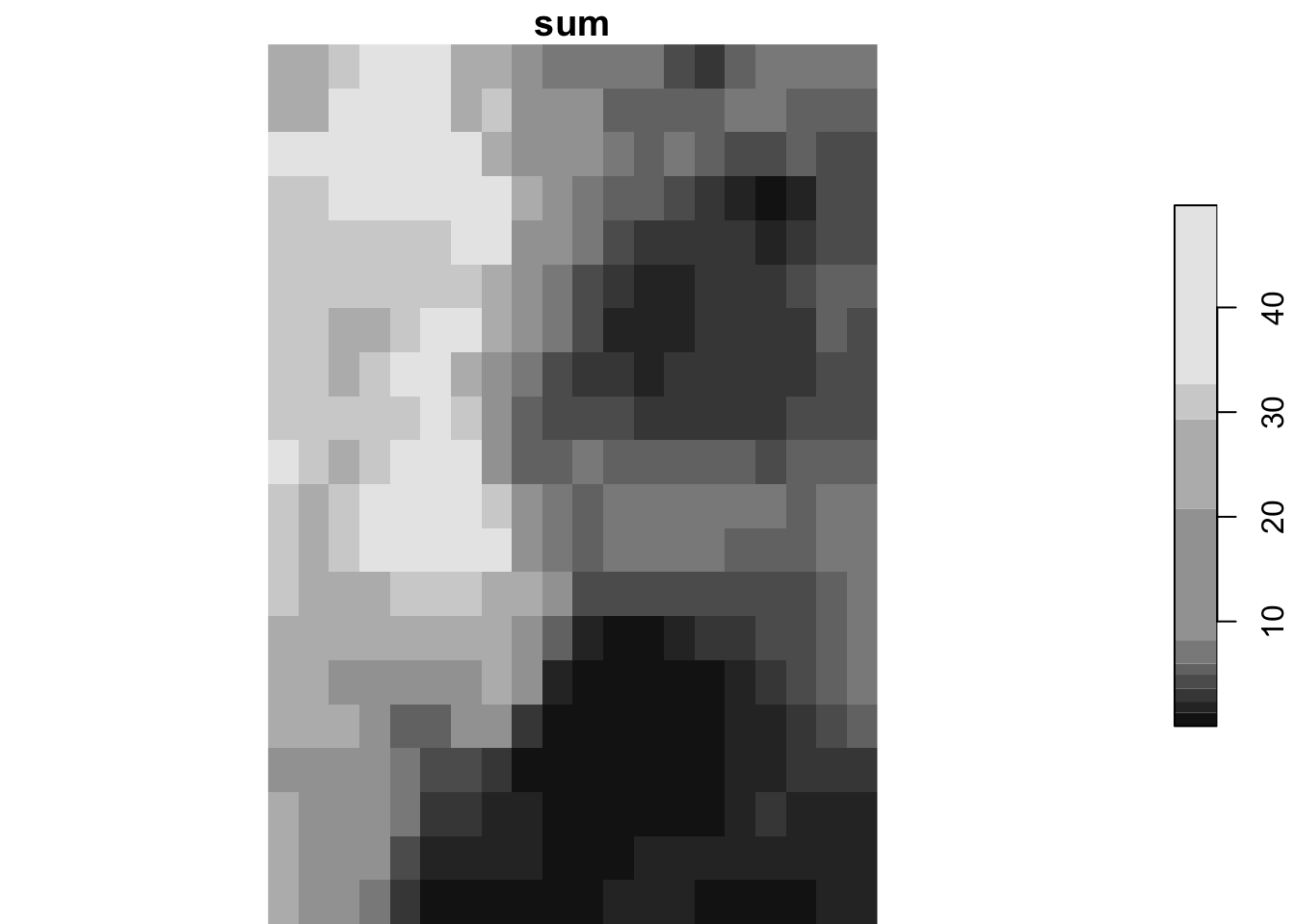
6.9 Convert from and to Raster\(^*\) or SpatRaster objects
When you need to convert a stars object to a Raster\(^*\) or SpatRaster object, you can use the as() function as follows:
(
  # to Raster* object
  prcp_tmax_PRISM_m8_y09_rb <- as(prcp_tmax_PRISM_m8_y09, "Raster")
)
class : RasterBrick
dimensions : 20, 20, 400, 10 (nrow, ncol, ncell, nlayers)
resolution : 0.04166667, 0.04166667 (x, y)
extent : -121.7292, -120.8958, 45.8125, 46.64583 (xmin, xmax, ymin, ymax)
crs : +proj=longlat +datum=NAD83 +no_defs
source : memory
names : layer.1, layer.2, layer.3, layer.4, layer.5, layer.6, layer.7, layer.8, layer.9, layer.10
min values : 0, 0, 0, 0, 0, 0, 0, 0, 0, 0
max values : 0.019, 18.888, 30.851, 4.287, 0.797, 0.003, 3.698, 1.801, 0.000, 0.000
time : 2009-08-11, 2009-08-12, 2009-08-13, 2009-08-14, 2009-08-15, 2009-08-16, 2009-08-17, 2009-08-18, 2009-08-19, 2009-08-20 (
# to SpatRaster
prcp_tmax_PRISM_m8_y09_sr <- as(prcp_tmax_PRISM_m8_y09, "SpatRaster")
)class : SpatRaster
dimensions : 20, 20, 10 (nrow, ncol, nlyr)
resolution : 0.04166667, 0.04166667 (x, y)
extent : -121.7292, -120.8958, 45.8125, 46.64583 (xmin, xmax, ymin, ymax)
coord. ref. : lon/lat NAD83 (EPSG:4269)
source(s) : memory
names : date2~08-11, date2~08-12, date2~08-13, date2~08-14, date2~08-15, date2~08-16, ...
min values : 0.000, 0.000, 0.000, 0.000, 0.000, 0.000, ...
max values : 0.019, 18.888, 30.851, 4.287, 0.797, 0.003, ... As you can see, date values in prcp_tmax_PRISM_m8_y09 appear in the time dimension of prcp_tmax_PRISM_m8_y09_rb (RasterBrick). However, in prcp_tmax_PRISM_m8_y09_sr (SpatRaster), date values appear in the names dimension with date added as prefix to the original date values.
Note also that the conversion was done for only the ppt attribute. This is simply because the raster and terra package does not accommodate multiple attributes of 3-dimensional array. So, if you want a RasterBrick or SpatRaster of the precipitation data, then you need to do the following:
(
  # to RasterBrick
  tmax_PRISM_m8_y09_rb <- as(prcp_tmax_PRISM_m8_y09["ppt", , , ], "Raster")
)
class : RasterBrick
dimensions : 20, 20, 400, 10 (nrow, ncol, ncell, nlayers)
resolution : 0.04166667, 0.04166667 (x, y)
extent : -121.7292, -120.8958, 45.8125, 46.64583 (xmin, xmax, ymin, ymax)
crs : +proj=longlat +datum=NAD83 +no_defs
source : memory
names : layer.1, layer.2, layer.3, layer.4, layer.5, layer.6, layer.7, layer.8, layer.9, layer.10
min values : 0, 0, 0, 0, 0, 0, 0, 0, 0, 0
max values : 0.019, 18.888, 30.851, 4.287, 0.797, 0.003, 3.698, 1.801, 0.000, 0.000
time : 2009-08-11, 2009-08-12, 2009-08-13, 2009-08-14, 2009-08-15, 2009-08-16, 2009-08-17, 2009-08-18, 2009-08-19, 2009-08-20 (
# to SpatRaster
tmax_PRISM_m8_y09_sr <- as(prcp_tmax_PRISM_m8_y09["ppt", , , ], "SpatRaster")
)class : SpatRaster
dimensions : 20, 20, 10 (nrow, ncol, nlyr)
resolution : 0.04166667, 0.04166667 (x, y)
extent : -121.7292, -120.8958, 45.8125, 46.64583 (xmin, xmax, ymin, ymax)
coord. ref. : lon/lat NAD83 (EPSG:4269)
source(s) : memory
names : date2~08-11, date2~08-12, date2~08-13, date2~08-14, date2~08-15, date2~08-16, ...
min values : 0.000, 0.000, 0.000, 0.000, 0.000, 0.000, ...
max values : 0.019, 18.888, 30.851, 4.287, 0.797, 0.003, ... You can convert a Raster\(^*\) object to a stars object using stars::st_as_stars() (you will see a use case in Section 8.4.2).
(
  tmax_PRISM_m8_y09_back_to_stars <- stars::st_as_stars(tmax_PRISM_m8_y09_rb)
)
stars object with 3 dimensions and 1 attribute
attribute(s):
Min. 1st Qu. Median Mean 3rd Qu. Max.
layer.1 0 0 0 1.292334 0.011 30.851
dimension(s):
from to offset delta refsys x/y
x 1 20 -121.7 0.04167 NAD83 [x]
y 1 20 46.65 -0.04167 NAD83 [y]
band 1 10 2009-08-11 1 days Date Notice that the original date values (stored in the date dimension) are recovered, but its dimension is now called just band.
You can do the same with a SpatRaster object.
(
  tmax_PRISM_m8_y09_back_to_stars <- stars::st_as_stars(tmax_PRISM_m8_y09_sr)
)
stars object with 3 dimensions and 1 attribute
attribute(s):
Min. 1st Qu. Median Mean 3rd Qu. Max.
date2009-08-11 0 0 0 1.292334 0.011 30.851
dimension(s):
from to offset delta refsys values x/y
x 1 20 -121.7 0.04167 NAD83 NULL [x]
y 1 20 46.65 -0.04167 NAD83 NULL [y]
band 1 10 NA NA NA date2009-08-11,...,date2009-08-20 Note that unlike the conversion from the RasterBrick object, the band dimension inherited values of the name dimension in tmax_PRISM_m8_y09_sr.
6.10 Spatial interactions of stars and sf objects
6.10.1 Spatial cropping (subsetting) to the area of interest
If the region of interest is smaller than the spatial extent of the stars raster data, there is no need to retain the irrelevant portions of the stars object. In such cases, you can crop the stars data to focus on the region of interest using sf::st_crop(). The general syntax of sf::st_crop() is:
#--- NOT RUN ---#
sf::st_crop(stars object, sf/bbox object)
For demonstration, we use PRISM tmax data for the U.S. for January 2019 as a stars object.
(
tmax_m8_y09_stars <-
  stars::read_stars("Data/PRISM_tmax_y2009_m8.tif") %>%
  setNames("tmax") %>%
  .[, , , 1:10] %>%
  stars::st_set_dimensions(
    "band",
    values = seq(
      lubridate::ymd("2009-08-01"),
      lubridate::ymd("2009-08-10"),
      by = "days"
    ),
    name = "date"
  )
)
stars object with 3 dimensions and 1 attribute
attribute(s), summary of first 1e+05 cells:
Min. 1st Qu. Median Mean 3rd Qu. Max. NA's
tmax 15.084 20.1775 22.584 23.86903 26.3285 41.247 60401
dimension(s):
from to offset delta refsys point x/y
x 1 1405 -125 0.04167 NAD83 FALSE [x]
y 1 621 49.94 -0.04167 NAD83 FALSE [y]
date 1 10 2009-08-01 1 days Date NA The region of interest is Michigan.
MI_county_sf <-
  tigris::counties(state = "Michigan", cb = TRUE, progress_bar = FALSE) %>%
  #--- transform using the CRS of the PRISM stars data  ---#
  sf::st_transform(sf::st_crs(tmax_m8_y09_stars))
We can crop the tmax data to the Michigan state border using st_crop() as follows:
(
tmax_MI <- sf::st_crop(tmax_m8_y09_stars, MI_county_sf)
)
stars object with 3 dimensions and 1 attribute
attribute(s):
Min. 1st Qu. Median Mean 3rd Qu. Max. NA's
tmax 14.108 22.471 24.343 24.61851 26.208 35.373 206900
dimension(s):
from to offset delta refsys point x/y
x 831 1023 -125 0.04167 NAD83 FALSE [x]
y 41 198 49.94 -0.04167 NAD83 FALSE [y]
date 1 10 2009-08-01 1 days Date NA Notice that from and to for x and y have changed to cover only the boundary box of the Michigan state border. Note that the values for the cells outside of the Michigan state border were set to NA. Figure 6.8 shows the cropping was successful.
plot(tmax_MI[,,,1])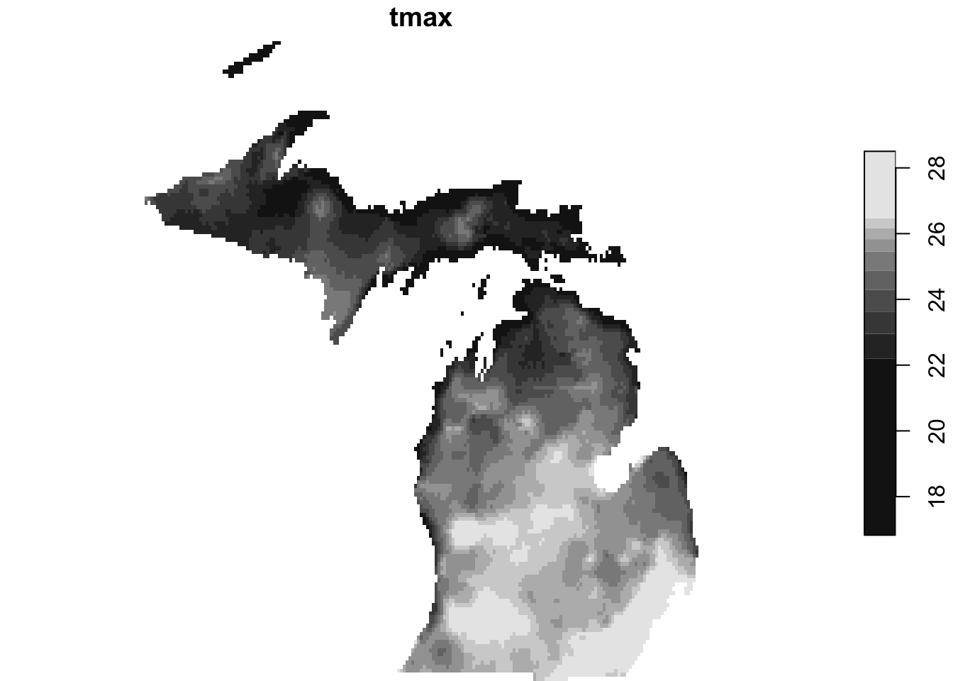
Alternatively, you could use [] like as follows to crop a stars object.
plot(tmax_m8_y09_stars[MI_county_sf])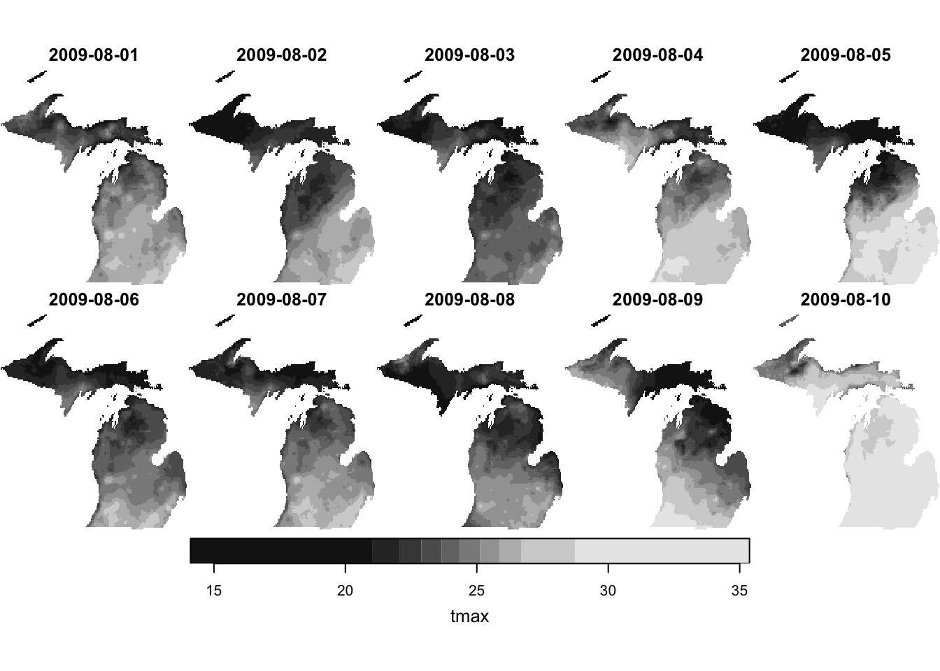
:::{.callout-note title = “Use bounding box”} When using sf::st_crop(), it is much faster to crop to a bounding box instead of sf if that is satisfactory. For example, you may be cropping a stars object to speed up subsequent raster value extraction (see Section 9.2). In this case, it is far better to crop to the bounding box of the sf instead of sf. Confirm the speed difference between the two below:
The difference can be substantial especially when the number of observations are large in sf. :::
6.10.2 Extracting values for points
In this section, we will learn how to extract cell values from raster layers as starts for spatial units represented as point sf data6.
6 see Section 5.2 for a detailed explanation of what it means to extract raster values.
6.10.2.1 Extraction using stars::st_extract()
For the illustrations in this section, we use the following datasets:
- Points: Irrigation wells in Kansas
- Raster: daily PRISM tmax data for August, 2009
PRISM tmax data
(
  tmax_m8_y09_stars <-
    stars::read_stars("Data/PRISM_tmax_y2009_m8.tif") %>%
    setNames("tmax") %>%
    .[, , , 1:10] %>%
    stars::st_set_dimensions(
      "band",
      values = seq(
        lubridate::ymd("2009-08-01"),
        lubridate::ymd("2009-08-10"),
        by = "days"
      ),
      name = "date"
    )
)
Irrigation wells in Kansas:
#--- read in the KS points data ---#
(
KS_wells <- readRDS("Data/Chap_5_wells_KS.rds")
)
Simple feature collection with 37647 features and 1 field
Geometry type: POINT
Dimension: XY
Bounding box: xmin: -102.0495 ymin: 36.99552 xmax: -94.62089 ymax: 40.00199
Geodetic CRS: NAD83
First 10 features:
well_id geometry
1 1 POINT (-100.4423 37.52046)
2 3 POINT (-100.7118 39.91526)
3 5 POINT (-99.15168 38.48849)
4 7 POINT (-101.8995 38.78077)
5 8 POINT (-100.7122 38.0731)
6 9 POINT (-97.70265 39.04055)
7 11 POINT (-101.7114 39.55035)
8 12 POINT (-95.97031 39.16121)
9 15 POINT (-98.30759 38.26787)
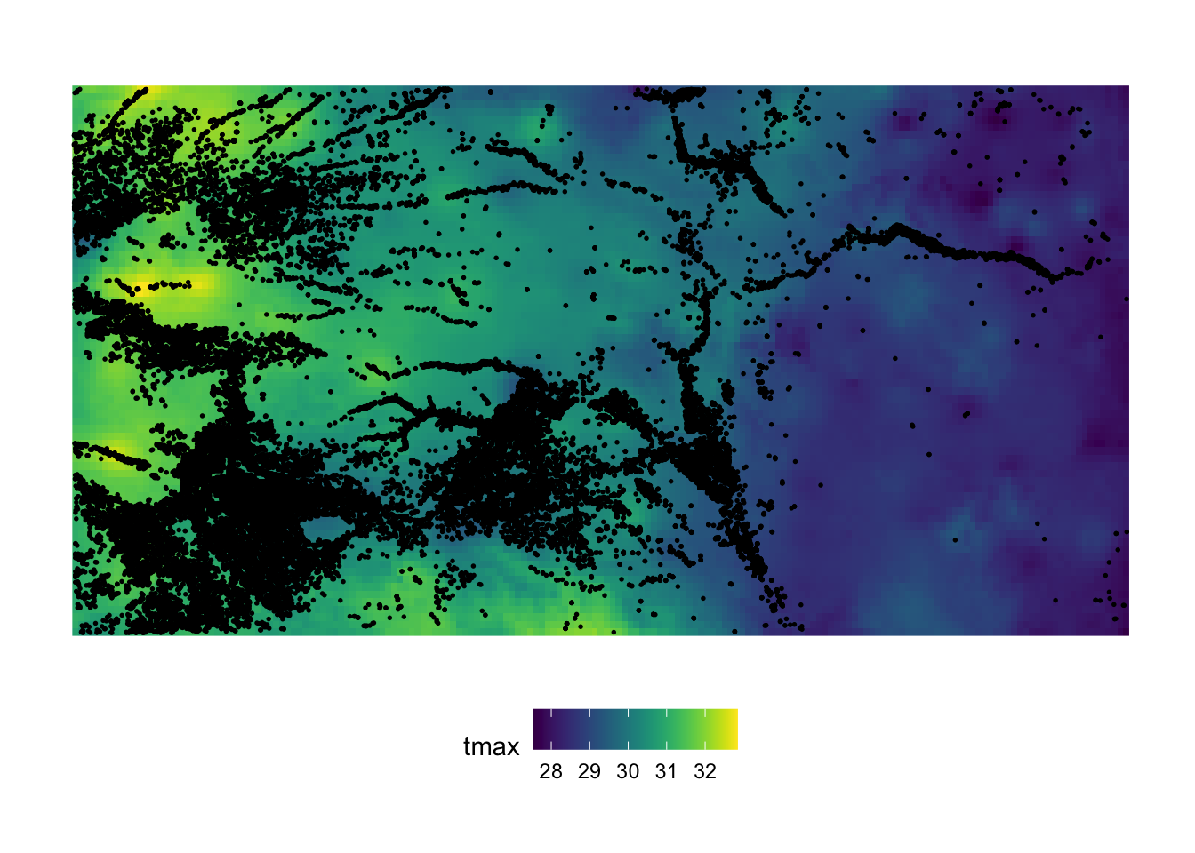
10 17 POINT (-100.2785 37.71539)Figure 6.9 show the spatial distribution of the irrigation wells over the PRISM grids:
Code
ggplot() +
  geom_stars(data = st_crop(tmax_m8_y09_stars[,,,1], st_bbox(KS_wells))) +
  scale_fill_viridis(name = "tmax") +
  geom_sf(data = st_transform(KS_wells, st_crs(tmax_m8_y09_stars)), size = 0.3) +
  theme_for_map +
  theme(
    legend.position = "bottom"
  )
We can extract the value of raster cells in which points are located using stars::st_extract().
#--- NOT RUN ---#
stars::st_extract(stars object, sf of points)
Before we extract values from the stars raster data, let’s crop it to the spatial extent of the KS_wells.
tmax_m8_y09_KS_stars <- sf::st_crop(tmax_m8_y09_stars, KS_wells)We also should change the CRS of KS_wells to that of tmax_m8_y09_KS_stars.
KS_wells <- sf::st_transform(KS_wells, sf::st_crs(tmax_m8_y09_stars))We now extract the value of rasters in which points are located:
(
extracted_tmax <- stars::st_extract(tmax_m8_y09_KS_stars, KS_wells)
)
stars object with 2 dimensions and 1 attribute
attribute(s):
Min. 1st Qu. Median Mean 3rd Qu. Max.
tmax 24.605 30.681 33.08 33.22354 36.38175 40.759
dimension(s):
from to offset delta refsys point
geometry 1 37647 NA NA NAD83 TRUE
date 1 10 2009-08-01 1 days Date NA
values
geometry POINT (-100.4423 37.52046),...,POINT (-99.96733 39.88535)
date NULLThe returned object is a stars object of simple features. You can convert this to a more familiar-looking sf object using sf::st_as_sf():
(
extracted_tmax_sf <- sf::st_as_sf(extracted_tmax)
)
Simple feature collection with 37647 features and 10 fields
Geometry type: POINT
Dimension: XY
Bounding box: xmin: -102.0495 ymin: 36.99552 xmax: -94.62089 ymax: 40.00199
Geodetic CRS: NAD83
First 10 features:
2009-08-01 2009-08-02 2009-08-03 2009-08-04 2009-08-05 2009-08-06 2009-08-07
1 30.131 27.070 32.288 37.496 33.977 32.563 33.733
2 31.533 28.373 35.927 36.942 30.557 31.235 31.121
3 30.591 27.968 33.279 38.182 33.783 32.790 29.852
4 31.307 27.565 34.945 38.056 32.832 30.040 31.744
5 30.715 27.836 33.458 38.083 33.912 31.895 32.497
6 29.661 27.592 32.192 36.787 33.856 31.655 29.434
7 31.308 27.876 35.709 36.806 32.254 29.634 31.048
8 28.776 25.930 30.293 34.316 30.861 29.100 29.051
9 30.583 26.527 32.315 37.495 32.576 31.702 28.578
10 29.715 27.051 32.638 37.328 33.863 32.001 33.281
2009-08-08 2009-08-09 2009-08-10 geometry
1 36.471 37.635 31.506 POINT (-100.4423 37.52046)
2 37.016 31.317 29.902 POINT (-100.7118 39.91526)
3 36.954 38.100 33.257 POINT (-99.15168 38.48849)
4 36.498 32.738 29.350 POINT (-101.8995 38.78077)
5 36.021 37.251 30.389 POINT (-100.7122 38.0731)
6 36.524 39.329 36.532 POINT (-97.70265 39.04055)
7 36.319 30.805 30.004 POINT (-101.7114 39.55035)
8 34.211 35.462 35.193 POINT (-95.97031 39.16121)
9 37.337 38.112 36.962 POINT (-98.30759 38.26787)
10 36.322 37.686 31.488 POINT (-100.2785 37.71539)As you can see each date forms a column of extracted values for the points because the third dimension of tmax_MI is date. So, you can easily turn the outcome to an sf object with date as Date object as follows.
(
extracted_tmax_long <-
  extracted_tmax_sf %>%
  tidyr::pivot_longer(- geometry, names_to = "date", values_to = "tmax") %>%
  sf::st_as_sf() %>%
  mutate(date = lubridate::ymd(date))
)
Simple feature collection with 376470 features and 2 fields
Geometry type: POINT
Dimension: XY
Bounding box: xmin: -102.0495 ymin: 36.99552 xmax: -94.62089 ymax: 40.00199
Geodetic CRS: NAD83
# A tibble: 376,470 × 3
geometry date tmax
* <POINT [°]> <date> <dbl>
1 (-100.4423 37.52046) 2009-08-01 30.1
2 (-100.4423 37.52046) 2009-08-02 27.1
3 (-100.4423 37.52046) 2009-08-03 32.3
4 (-100.4423 37.52046) 2009-08-04 37.5
5 (-100.4423 37.52046) 2009-08-05 34.0
6 (-100.4423 37.52046) 2009-08-06 32.6
7 (-100.4423 37.52046) 2009-08-07 33.7
8 (-100.4423 37.52046) 2009-08-08 36.5
9 (-100.4423 37.52046) 2009-08-09 37.6
10 (-100.4423 37.52046) 2009-08-10 31.5
# ℹ 376,460 more rowsNote that all the variables other than geometry in the points data (KS_wells) are lost at the time of applying stars::st_extract(). You take advantage the fact that the the order of the observations in the object returned by stars::st_extract() is the order of the points (KS_wells).
(
extracted_tmax_long <-
  extracted_tmax_sf %>%
  mutate(well_id = KS_wells$well_id) %>%
  pivot_longer(c(- geometry, - well_id), names_to = "date", values_to = "tmax") %>%
  st_as_sf() %>%
  mutate(date = ymd(date))
)
Simple feature collection with 376470 features and 3 fields
Geometry type: POINT
Dimension: XY
Bounding box: xmin: -102.0495 ymin: 36.99552 xmax: -94.62089 ymax: 40.00199
Geodetic CRS: NAD83
# A tibble: 376,470 × 4
geometry well_id date tmax
* <POINT [°]> <dbl> <date> <dbl>
1 (-100.4423 37.52046) 1 2009-08-01 30.1
2 (-100.4423 37.52046) 1 2009-08-02 27.1
3 (-100.4423 37.52046) 1 2009-08-03 32.3
4 (-100.4423 37.52046) 1 2009-08-04 37.5
5 (-100.4423 37.52046) 1 2009-08-05 34.0
6 (-100.4423 37.52046) 1 2009-08-06 32.6
7 (-100.4423 37.52046) 1 2009-08-07 33.7
8 (-100.4423 37.52046) 1 2009-08-08 36.5
9 (-100.4423 37.52046) 1 2009-08-09 37.6
10 (-100.4423 37.52046) 1 2009-08-10 31.5
# ℹ 376,460 more rowsWe can now summarize the data by well_id and then merge it back to KS_wells.
KS_wells <-
  extracted_tmax_long %>%
  #--- geometry no longer needed ---#
  # if you do not do this, summarize() takes a long time
  sf::st_drop_geometry() %>%
  dplyr::group_by(well_id, month(date)) %>%
  dplyr::summarize(mean(tmax)) %>%
  dplyr::left_join(KS_wells, ., by = "well_id")
6.10.3 Extract and summarize values for polygons
In this section, we will learn how to extract cell values from raster layers as starts for spatial units represented as polygons sf data (see Section 5.2 for a more detailed explanation of this operation).
In order to extract cell values from stars objects (just like Chapter 5) and summarize them for polygons, you can use aggregate.stars(). Although introduced here because it natively accepts stars objects, aggregate.stars() is not recommended unless the raster data is small (with a small number of cells). It is almost always slower than the two other alternatives: terra::extract() and exactextractr::exact_extract() even though they involve conversion of stars objects to SpatRaster objects. For a comparison of its performance relative to these alternatives, see Section 9.3. If you just want to see the better alternatives, you can just skip to Section 6.10.3.2.
6.10.3.1 aggregate.stars()
The syntax of aggregate.stars() is as follows:
#--- NOT RUN ---#
aggregate(stars object, sf object, FUN = function to apply)
For each polygon, aggregate() identifies the cells whose centroids lie within the polygon, extracts their values, and applies the specified function to those values. Let’s now see a demonstration of how to use aggregate(). For this example, we will use Kansas counties as the polygon data.
KS_county_sf <-
tigris::counties(state = "Kansas", cb = TRUE, progress_bar = FALSE)%>%
#--- transform using the CRS of the PRISM stars data ---#
sf::st_transform(sf::st_crs(tmax_m8_y09_stars)) %>%
#--- generate unique id ---#
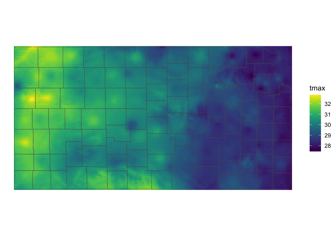
dplyr::mutate(id = 1:nrow(.))Figure 6.10 shows polygons (counties) superimposed on top of the tmax raster data:
For example, the following code will find the mean of the tmax values for each county:
(
mean_tmax_stars <- aggregate(tmax_m8_y09_stars, KS_county_sf, FUN = mean)
)
stars object with 2 dimensions and 1 attribute
attribute(s):
Min. 1st Qu. Median Mean 3rd Qu. Max.
tmax 24.91317 29.65889 32.56404 32.5487 35.34826 39.70888
dimension(s):
from to offset delta refsys point
geometry 1 105 NA NA NAD83 FALSE
date 1 10 2009-08-01 1 days Date NA
values
geometry MULTIPOLYGON (((-101.0681...,...,MULTIPOLYGON (((-96.50168...
date NULLAs you can see, the aggregate() operation also returns a stars object for polygons just like stars::st_extract() did. You can convert the stars object into an sf object using sf::st_as_sf():
mean_tmax_sf <- sf::st_as_sf(mean_tmax_stars)As you can see, aggregate() function extracted values for the polygons from all the layers across the date dimension, and the values from individual dates become variables where the variables names are the corresponding date values.
Just like the case of raster data extraction for points data we saw in Section 6.10.2, no information from the polygons (KS_county_sf) except the geometry column remains. For further processing of the extracted data and easy merging with the polygons data (KS_county_sf), we can assign the unique county id just like we did for the case of points data.
(
  mean_tmax_long <-
    mean_tmax_sf %>%
    #--- drop geometry ---#
    sf::st_drop_geometry() %>%
    #--- assign id before transformation ---#
    dplyr::mutate(id = KS_county_sf$id) %>%
    #--- then transform ---#
    tidyr::pivot_longer(-id, names_to = "date", values_to = "tmax")
)
aggregate() will return NA for polygons that intersect with raster cells that have NA values. To ignore the NA values when applying a function, we can add na.rm=TRUE option like this:
6.10.3.2 exactextractr::exact_extract()
A great alternative to aggregate() is to extract raster cell values using exactextractr::exact_extract() or terra::extract() and then summarize the results yourself. Both are considerably faster than aggregate.stars(). Although they do not natively accept stars objects, you can easily convert a stars object to a SpatRaster using as(stars, "SpatRaster") and then use these methods.
Let’s first convert tmax_m8_y09_KS_stars (a stars object) into a SpatRaster object.
(
tmax_m8_y09_KS_sr <- as(tmax_m8_y09_KS_stars, "SpatRaster")
)
class : SpatRaster
dimensions : 73, 179, 10 (nrow, ncol, nlyr)
resolution : 0.04166667, 0.04166667 (x, y)
extent : -102.0625, -94.60417, 36.97917, 40.02083 (xmin, xmax, ymin, ymax)
coord. ref. : lon/lat NAD83 (EPSG:4269)
source(s) : memory
names : date2~08-01, date2~08-02, date2~08-03, date2~08-04, date2~08-05, date2~08-06, ...
min values : 27.639, 24.605, 28.094, 32.711, 28.972, 26.871, ...
max values : 32.844, 32.341, 37.560, 40.759, 39.466, 36.303, ... Now, we can use exactextractr::exact_extract() as follows:
extracted_values <- exactextractr::exact_extract(tmax_m8_y09_KS_sr, KS_county_sf, include_cols = "COUNTYFP")The returned outcome is a list of data.frame. Let’s take a look at the first 6 rows of the first 3 elements of the list.
extracted_values[1:3] %>% lapply(., head)[[1]]
COUNTYFP date2009-08-01 date2009-08-02 date2009-08-03 date2009-08-04
1 175 30.954 27.629 34.411 37.547
2 175 NA NA NA NA
3 175 30.866 27.506 34.229 37.464
4 175 30.837 27.398 34.126 37.364
5 175 30.759 27.369 33.969 37.323
6 175 30.584 27.399 33.734 37.284
date2009-08-05 date2009-08-06 date2009-08-07 date2009-08-08 date2009-08-09
1 34.264 33.468 35.103 36.674 37.961
2 NA NA NA NA NA
3 34.217 33.348 34.925 36.552 37.861
4 34.198 33.314 34.860 36.442 37.762
5 34.159 33.186 34.728 36.463 37.778
6 34.098 33.092 34.512 36.487 37.723
date2009-08-10 coverage_fraction
1 31.715 0.1074141
2 NA 0.8066747
3 31.564 0.8066615
4 31.432 0.8066448
5 31.463 0.8061629
6 31.592 0.8054324
[[2]]
COUNTYFP date2009-08-01 date2009-08-02 date2009-08-03 date2009-08-04
1 027 29.623 26.370 32.274 35.627
2 027 29.657 26.306 32.209 35.527
3 027 29.665 26.254 32.213 35.421
4 027 NA NA NA NA
5 027 NA NA NA NA
6 027 NA NA NA NA
date2009-08-05 date2009-08-06 date2009-08-07 date2009-08-08 date2009-08-09
1 31.836 30.141 29.131 35.980 38.073
2 31.787 30.081 29.089 35.968 37.983
3 31.719 30.010 29.049 35.951 37.949
4 NA NA NA NA NA
5 NA NA NA NA NA
6 NA NA NA NA NA
date2009-08-10 coverage_fraction
1 34.794 0.03732148
2 34.905 0.10592906
3 34.810 0.10249268
4 NA 0.10018899
5 NA 0.10074520
6 NA 0.09701102
[[3]]
COUNTYFP date2009-08-01 date2009-08-02 date2009-08-03 date2009-08-04
1 171 NA NA NA NA
2 171 NA NA NA NA
3 171 NA NA NA NA
4 171 NA NA NA NA
5 171 NA NA NA NA
6 171 NA NA NA NA
date2009-08-05 date2009-08-06 date2009-08-07 date2009-08-08 date2009-08-09
1 NA NA NA NA NA
2 NA NA NA NA NA
3 NA NA NA NA NA
4 NA NA NA NA NA
5 NA NA NA NA NA
6 NA NA NA NA NA
date2009-08-10 coverage_fraction
1 NA 0.1813289
2 NA 0.3062004
3 NA 0.2972469
4 NA 0.2887933
5 NA 0.2825042
6 NA 0.2799884As you can see, each data.frame has variables called COUNTYFP, date2009-08-01, \(\dots\), date2009-08-10 (they are from the layer names in tmax_m8_y09_KS_sr) and coverage_fraction. COUNTYFP was inherited from KS_county_sf thanks to include_cols = "COUNTYFP" and let us merge the extracted values with KS_county_sf.
In order to make the results easier to work with, you can process them to get a single data.frame, taking advantage of dplyr::bind_rows() to combine the list of the datasets into one dataset.
extracted_values_df <-
  extracted_values %>%
  #--- combine the list of data.frames ---#
  dplyr::bind_rows()

head(extracted_values_df)
COUNTYFP date2009-08-01 date2009-08-02 date2009-08-03 date2009-08-04
1 175 30.954 27.629 34.411 37.547
2 175 NA NA NA NA
3 175 30.866 27.506 34.229 37.464
4 175 30.837 27.398 34.126 37.364
5 175 30.759 27.369 33.969 37.323
6 175 30.584 27.399 33.734 37.284
date2009-08-05 date2009-08-06 date2009-08-07 date2009-08-08 date2009-08-09
1 34.264 33.468 35.103 36.674 37.961
2 NA NA NA NA NA
3 34.217 33.348 34.925 36.552 37.861
4 34.198 33.314 34.860 36.442 37.762
5 34.159 33.186 34.728 36.463 37.778
6 34.098 33.092 34.512 36.487 37.723
date2009-08-10 coverage_fraction
1 31.715 0.1074141
2 NA 0.8066747
3 31.564 0.8066615
4 31.432 0.8066448
5 31.463 0.8061629
6 31.592 0.8054324Now, let’s find area-weighted mean of tmax for each of the county-date combinations. The following code
- reshapes
extracted_values_dfto a long format - recovers date as
Dateobject - calculates area-weighted mean of tmax by county-date
extracted_values_df %>%
  #--- long to wide ---#
  tidyr::pivot_longer(
    c(-COUNTYFP, -coverage_fraction),
    names_to = "date",
    values_to = "tmax"
  ) %>%
  #--- remove date  ---#
  dplyr::mutate(
    #--- remove "date" from date and then convert it to Date ---#
    date = gsub("date", "", date) %>% lubridate::ymd()
  ) %>%
  #--- mean area-weighted tmax by county-date ---#
  dplyr::group_by(COUNTYFP, date) %>%
  na.omit() %>%
  dplyr::summarize(sum(tmax * coverage_fraction)/sum(coverage_fraction))
# A tibble: 960 × 3
# Groups: COUNTYFP [96]
COUNTYFP date `sum(tmax * coverage_fraction)/sum(coverage_fraction)`
<chr> <date> <dbl>
1 005 2009-08-01 28.2
2 005 2009-08-02 26.0
3 005 2009-08-03 29.3
4 005 2009-08-04 33.6
5 005 2009-08-05 30.4
6 005 2009-08-06 28.1
7 005 2009-08-07 28.9
8 005 2009-08-08 33.3
9 005 2009-08-09 34.8
10 005 2009-08-10 34.4
# ℹ 950 more rowsThis can now be readily merged with KS_county_sf using COUNTYFP as the key.
6.10.3.3 Summarizing the extracted values inside exactextractr::exact_extract()
Instead of returning the value from all the intersecting cells, exactextractr::exact_extract() can summarize the extracted values by polygon and then return the summarized numbers. This is much like how aggregate() works, which we saw above. There are multiple default options you can choose from. All you need to do is to add the desired summary function name as the third argument of exactextractr::exact_extract(). For example, the following will get us the mean of the extracted values weighted by coverage_fraction.
extacted_mean <- exactextractr::exact_extract(tmax_m8_y09_KS_sr, KS_county_sf, "mean", append_cols = "COUNTYFP", progress = FALSE)

head(extacted_mean)
Notice that you use append_cols instead of include_cols when you summarize within exactextractr::exact_extract().
(
mean_tmax_long <-
  extacted_mean %>%
  #--- wide to long ---#
  pivot_longer(-COUNTYFP, names_to = "date", values_to = "tmax") %>%
  #--- recover date ---#
  dplyr::mutate(date = gsub("mean.date", "", date) %>% lubridate::ymd())
)
# A tibble: 1,050 × 3
COUNTYFP date tmax
<chr> <date> <dbl>
1 175 2009-08-01 30.8
2 175 2009-08-02 27.7
3 175 2009-08-03 34.0
4 175 2009-08-04 37.2
5 175 2009-08-05 34.8
6 175 2009-08-06 33.9
7 175 2009-08-07 35.2
8 175 2009-08-08 36.8
9 175 2009-08-09 38.0
10 175 2009-08-10 32.3
# ℹ 1,040 more rowsThere are other summary function options that may be of interest, such as “max”, “min.” You can see all the default options at the package website.
6.10.3.4 area-weighted v.s. coverage-fraction-weighted summary (Optional)
When we found the mean of tmax weighted by coverage fraction, each raster cell was assumed to cover the same area. This is not exactly correct when a raster layer in geographic coordinates (latitude/longitude) is used. To see this, let’s find the area of each cell using terra::cellSize().
(
raster_area_data <- terra::cellSize(tmax_m8_y09_KS_sr)
)
class : SpatRaster
dimensions : 73, 179, 1 (nrow, ncol, nlyr)
resolution : 0.04166667, 0.04166667 (x, y)
extent : -102.0625, -94.60417, 36.97917, 40.02083 (xmin, xmax, ymin, ymax)
coord. ref. : lon/lat NAD83 (EPSG:4269)
source(s) : memory
name : area
min value : 16461242
max value : 17149835 The output is a SpatRaster, where the area of the cells are stored as values. Figure 6.11 shows the map of the PRISM raster cells in Kansas, color-differentiated by area.
Code
plot(raster_area_data)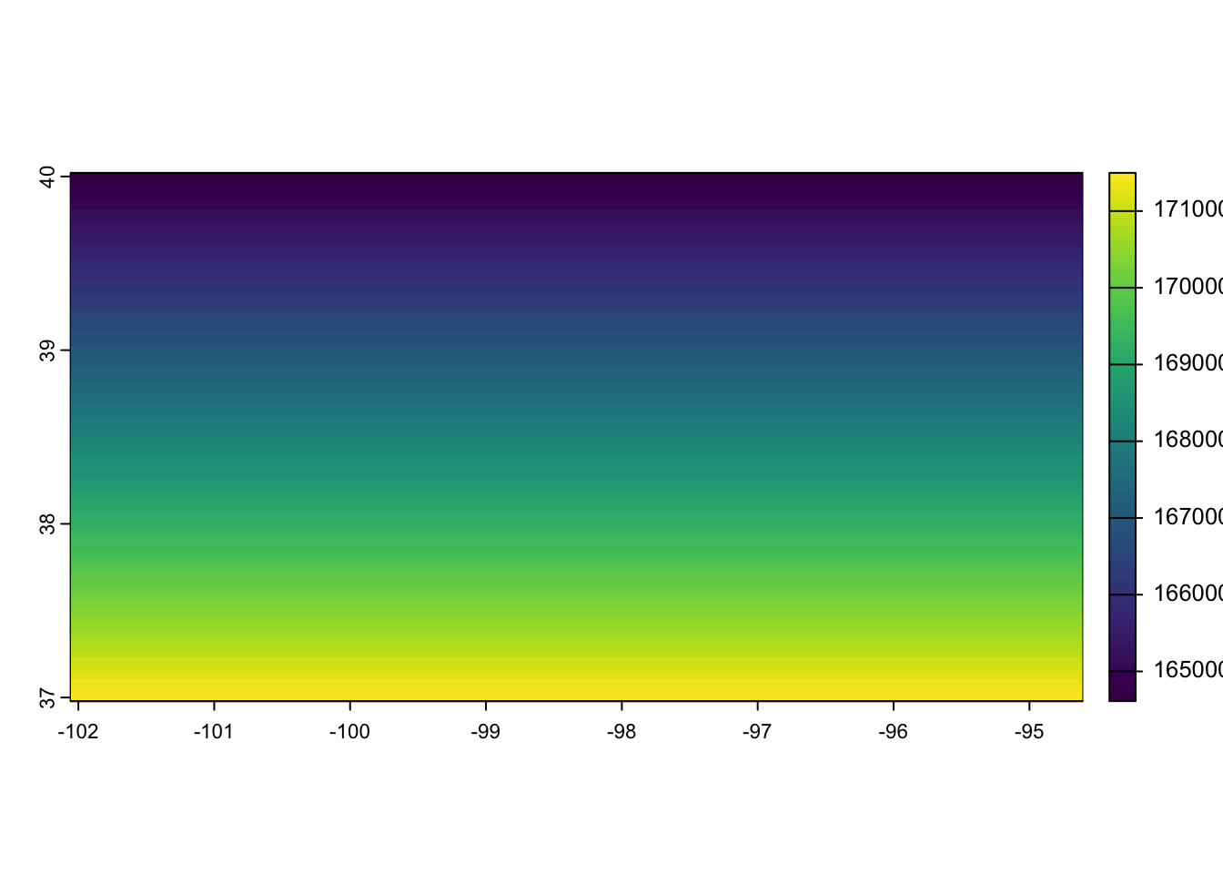
The area of a raster cell becomes slightly larger as the latitude increases. This is mainly due to the fact that 1 degree in longitude is longer in actual length on the earth surface at a higher latitude than at a lower latitude in the northern hemisphere.7 The mean of extracted values weighted by coverage fraction ignores this fact and implicitly assumes the all the cells have the same area.
7 The opposite happens in the southern hemisphere.
In order to get an area-weighted mean instead of a coverage-weighted mean, you can use the “weighted_mean” option as the third argument and also supply the SpatRaster of area (raster_area_data here) like this:
extracted_weighted_mean <-
  exactextractr::exact_extract(
    tmax_m8_y09_KS_sr,
    KS_county_sf,
    "weighted_mean",
    weights = raster_area_data,
    append_cols = "COUNTYFP",
    progress = FALSE
  )
Let’s compare the difference in the calculated means from the two methods for the first polygon.
extracted_weighted_mean[, 2] - extacted_mean[, 2] [1] 1.316071e-04 -8.201599e-05 -1.201630e-04 -1.029968e-04 3.585815e-04
[6] 8.010864e-05 -2.212524e-04 -1.335144e-05 -8.392334e-05 -1.640320e-04
[11] -7.057190e-05 -4.386902e-05 -1.850128e-04 -1.506805e-04 6.504059e-04
[16] 1.983643e-04 0.000000e+00 3.623962e-04 8.201599e-05 3.509521e-04
[21] 3.814697e-06 1.258850e-04 -1.602173e-04 -9.155273e-05 -7.247925e-05
[26] -4.768372e-05 0.000000e+00 -2.861023e-05 -4.005432e-05 4.577637e-05
[31] 1.716614e-05 1.869202e-04 5.340576e-05 -4.386902e-05 1.621246e-04
[36] -2.365112e-04 3.814697e-05 2.803802e-04 -4.005432e-05 NaN
[41] 6.103516e-05 4.005432e-05 7.629395e-05 -1.392365e-04 2.593994e-04
[46] 3.623962e-05 -3.814697e-05 -3.814697e-05 4.386902e-05 -1.907349e-06
[51] 2.670288e-04 6.675720e-05 3.623962e-04 4.005432e-04 -1.029968e-04
[56] -1.010895e-04 -7.247925e-05 0.000000e+00 -6.294250e-05 -7.629395e-06
[61] NaN -3.147125e-04 -5.149841e-05 -4.768372e-05 -1.487732e-04
[66] -9.155273e-05 NaN 8.773804e-05 -1.525879e-05 -3.204346e-04
[71] NaN -5.531311e-04 5.722046e-06 1.201630e-03 6.866455e-05
[76] -6.294250e-05 -7.629395e-06 -1.907349e-05 1.964569e-04 -1.869202e-04
[81] -1.125336e-04 2.803802e-04 2.861023e-05 -1.964569e-04 NaN
[86] -9.536743e-06 7.057190e-05 -2.536774e-04 -4.005432e-05 -3.623962e-05
[91] -1.945496e-04 -2.593994e-04 -1.029968e-04 NaN NaN
[96] 4.959106e-05 -5.531311e-05 NaN -6.866455e-05 7.762909e-04
[101] 1.010895e-04 -7.629395e-06 5.531311e-05 NaN -8.392334e-05As you can see the error is minimal. So, the consequence of using coverage-weighted means should be negligible in most cases. Indeed, unless polygons span a wide range of latitude and longitude, the error introduce by using the coverage-weighted mean instead of area-weighted mean should be negligible.
Pebesma, Edzer. 2020. Stars: Spatiotemporal Arrays, Raster and Vector Data Cubes. https://CRAN.R-project.org/package=stars.