7 Rmarkdown-PDF
7.1 Before you start
To author a full journal article in PDF using Rmarkdown, you will need to acquire or have familiarity with the following skills:
Before delving into this chapter, carefully consider the time and effort required to master these skills. Ensure the investment aligns with your goals and priorities.
While you can generate a PDF article without LaTeX expertise, it’s strongly advised to familiarize yourself with LaTeX debugging. This not only aids in customizing the article format but also prepares you for potential compilation errors you might face.
7.2 Preparation
Before diving in, please do the followings:
Go here and download all the files including sample_to_pdf.rmd, which we refer to as the sample rmd file throughout this chapter. Alternatively, you can clone this Github repository.
Knit sample_to_pdf.rmd to produce sample_to_pdf.pdf, which we refer to as the sample PDF file.
Install the following packages if you have not
knitrRmarkdowntidyversemodelsummarygtsummaryhuxtablekableExtra
7.3 Setting up a Quarto file with YAML
An Rmarkdown file starts with a YAML header, which lets you specify things like
- paper title
- authors (with affiliations and other subsidiary information)
- date
- abstract
It also lets you specify various aspects of the output PDF file including
- whether to include table of contents (
toc) - the depth of table of contents (
toc_depth) - whether to number sections or not (
number_sections) - how to display plots
- size
- alignment
This is also where you specify what files you use as bibliography, citation style, among other things. Important ones will be introduced later.
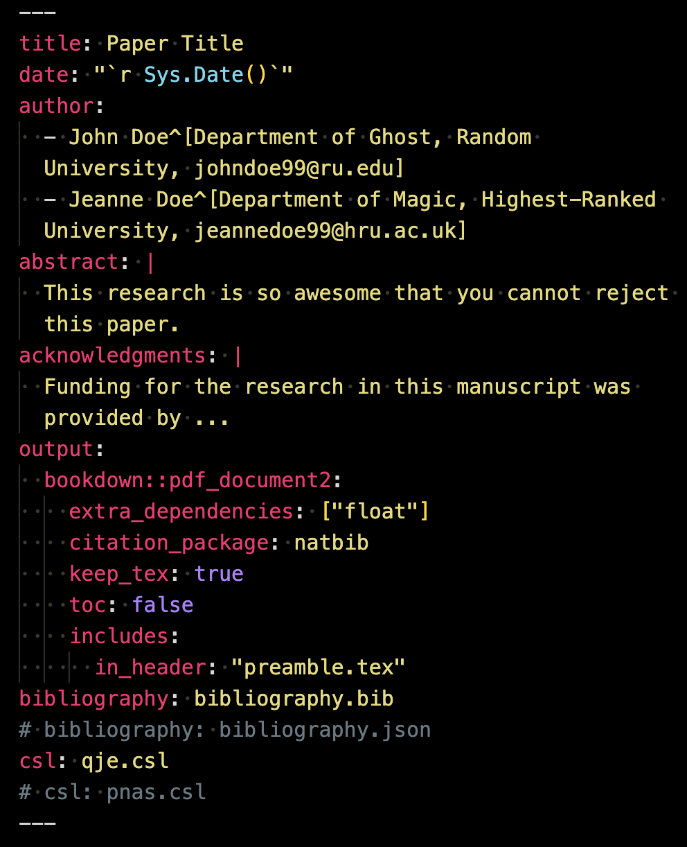
Here is an example YAML header, which you can see in sample_to_pdf.rmd file.
Full list of options can be found here. More detailed explanation of some of the output options will be provided later individually when the relevant topics are discussed.
Note that we are using bookdown::pdf_document2 from the bookdown package instead of using pdf_document from the Rmarkdown package. The use of bookdown::pdf_document2 enables cross-referencing of tables.
7.4 Using existing journal templates
Before anything, you should first check if the collection of templates provided by the rticles package has the template for your target journal.
Here are the currently available templates offered by the package (You can also see a more informative version of the list on the package GitHub site.).
rticles::journals() [1] "acm" "acs" "aea" "agu"
[5] "ajs" "amq" "ams" "arxiv"
[9] "asa" "bioinformatics" "biometrics" "copernicus"
[13] "ctex" "elsevier" "frontiers" "glossa"
[17] "ieee" "ims" "informs" "iop"
[21] "isba" "jasa" "jedm" "joss"
[25] "jss" "lipics" "lncs" "mdpi"
[29] "mnras" "oup_v0" "oup_v1" "peerj"
[33] "pihph" "plos" "pnas" "rjournal"
[37] "rsos" "rss" "sage" "sim"
[41] "springer" "tf" "trb" "wellcomeor" To start a template, click on the button with green plus on a white sheet of paper at the left upper corner of the RStudio IDE and select R Markdown as shown below:
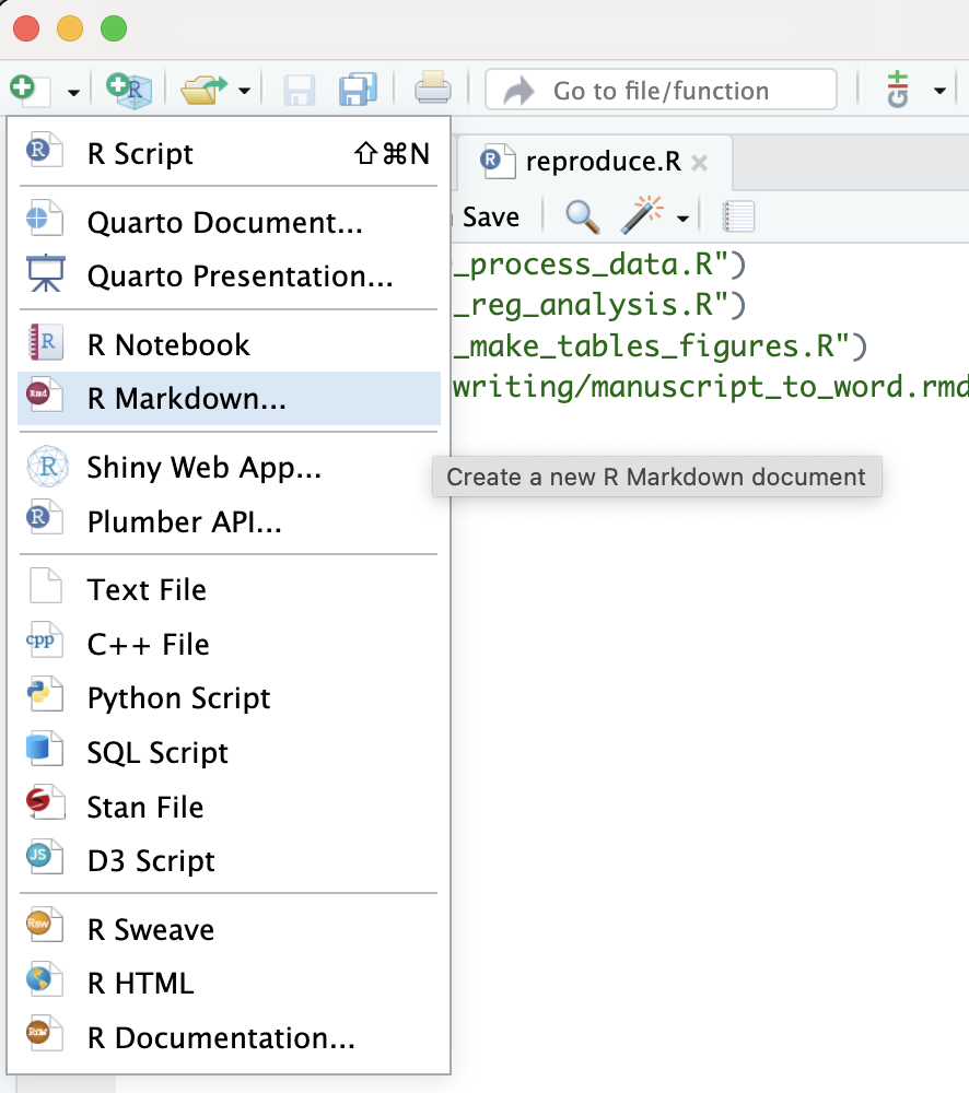
You can then select From Template, pick the template you would like to use, give the new directory a name, and hit OK.
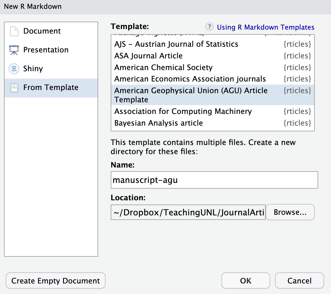
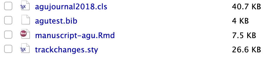
You will see a folder and a .Rproj. In the folder, you will find a template Rmarkdown file and other assets that are necessary for compiling the Rmarkdown file into the journal format.
7.5 Problems
https://stackoverflow.com/questions/77290665/did-i-break-r-markdown-every-file-i-try-gives-the-error-undefined-control-se
7.6 Citations and References
7.6.1 Set up
Begin by preparing a file that contains all your references. In your document’s YAML header, specify the bibliography file:
bibliography: bibliography file nameThere are multiple formats and systems available for bibliographies, such as BibLaTeX/BibTex (.bib), CSL-JSON (.json), and EndNote (.enl). among others.
In this illustration, we are employing a .bib file. If our bibliography file is titled bibliography.bib, the YAML header would look like:

When knitting to PDF, the references will be positioned at the conclusion of the document, as documented (see here). Append # References {-} to the tail end of your .qmd file. This creates a “References” section heading where all the citations will be listed. Including {-} adjacent to the section header ensures the References section remains unnumbered. This is particularly useful if you have activated section numbering in the YAML header with number-sections: true. Without {-}, the “References” section would be automatically numbered, which is often not desired in academic and professional documents.
7.6.2 Cite and create references
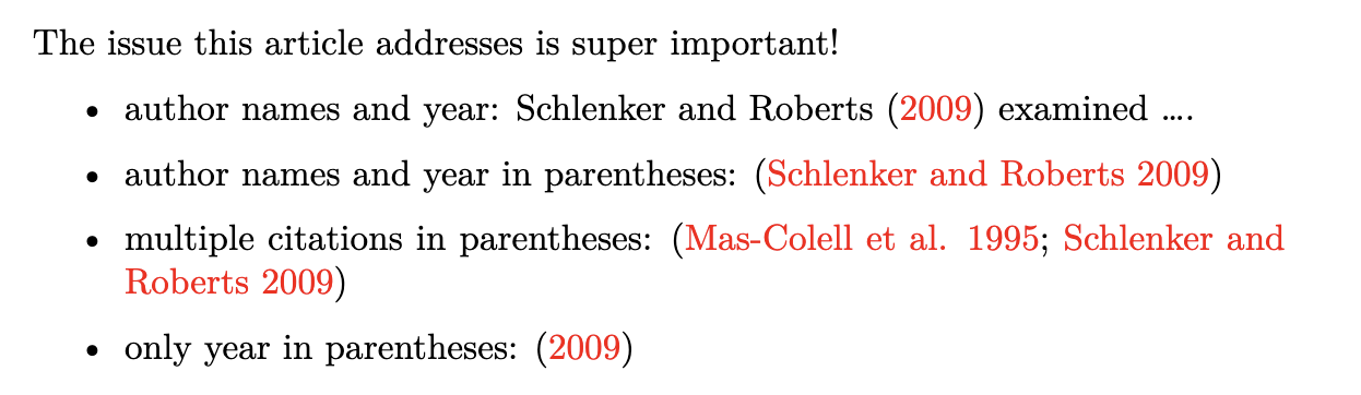
To cite, use the following syntax:
@reference_nameto print “author names (year)” in the output WORD file[@reference_name]to print “(author names, year)” in the output WORD file[@reference_name_1; @reference_name_2]to print “(author names, year; author names, year)” in the output WORD file[-@reference_name]to print just year
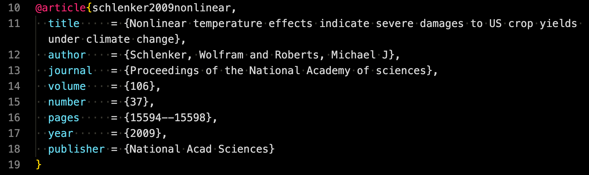
reference_name is the very first entry of a .bib file as in
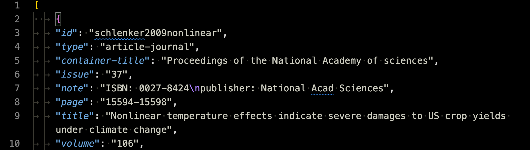
If you are using CSL json file, then it is the id of an entry as in
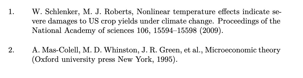
The cited items are automatically added to the reference following the specified style (see the next section).
7.6.3 Citation and Reference Style
You can change the citation and reference style using Citation Style Language. Citation style files have .csl extension.
Obtain the csl file you would like to use from the Zotero citation style repository.
Place the following in the YAML header:
csl: csl file name - Then, when knitted, citations and references styles reflect the style specified by the csl file
Currently, the csl style is set to qje.csl (citation style language for The Quarterly Journal of Economics) as below
Citation and references styles in the output PDF file follows the rules for the QJE.

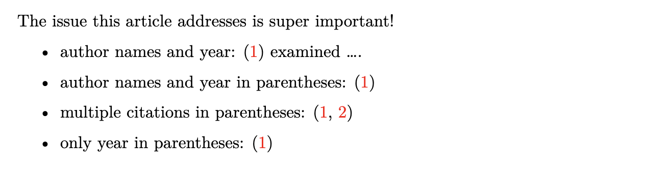
Now, comment csl: qje.csl and uncomment csl: pnas.csl so that the CSL for the Proceedings of the National Academy of Sciences (PNAS) is used, and then knit the sample qmd file.
You can now see that the citation style no longer respects the rules I mentioned above and also the reference style follows that of PNAS. This is because PNAS uses only numbers, but not author names or years.
7.7 Tables (Cross-referenced)
Create a table using any R package that can produce latex tables.
Add an R code chunk like this:
```{r tbl-id}
table_sample
```table_sampleis the name of the table created on R.tbl-idis the R chunk label you can use to cross-reference the table
- Use
\@ref(tab:tbl-id)in the Rmarkdown file to cross-reference the table (table numbering in the output PDF file is automatic).
7.7.1 Packages to create tables
7.7.1.1 Simple table from a data.frame
There are many R packages that let you create tables that are compatible with Latex. For example, you can use the kableExtra and huxtable package to create tables from a data.frame-like R objects from scratch. Here is an example code using the huxtable package.
library(huxtable)

head(iris, 10) %>%
# Create a huxtable
as_hux() %>%
# Add some basic styling
set_background_color(row = 1, value = "lightgray") %>% # Background color for header
set_caption("This is how you add the caption")
The gt package does not work as well with Latex as it does with the html output1. In academic journals, fancy looking tables are not necessary. kableExtra and huxtable are likely to be very much sufficient.
7.7.1.2 Regressions results and summary tables
For regression results and summary statics, the modelsummary and gtsummary2 packages are particularly convenient and useful. For example, the modelsummary package lets you create regression results and summary statistics tables via the modelsummary() function and summary statistics tables via the datasummary() function3. For the gtsummary package, their respective corresponding functions are tbl_regression and tbl_summary. For regression results tables, the stargazer package is also a viable option. It is less capable in creating summary statistics tables than modelsummary and gtsummary.
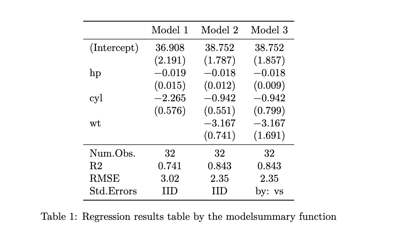
Here are example R codes that use the modelsummary package to create regression results and summary statistics tables.
Regression table
#--- regressions ---#
lm_1 <- fixest::feols(mpg ~ hp + cyl, data = mtcars)
lm_2 <- fixest::feols(mpg ~ hp + cyl + wt, data = mtcars)
lm_3 <- fixest::feols(mpg ~ hp + cyl + wt, cluster = ~ vs, data = mtcars)

#--- create a regression results table ---#
library(modelsummary)

modelsummary(
  list(lm_1, lm_2, lm_3),
  gof_omit = "IC|Log|Adj|F|Pseudo|Within",
  #--- add the title (caption) here ---#
  title = "Reression Results"
)
This is how the table would appear on the output PDF file.
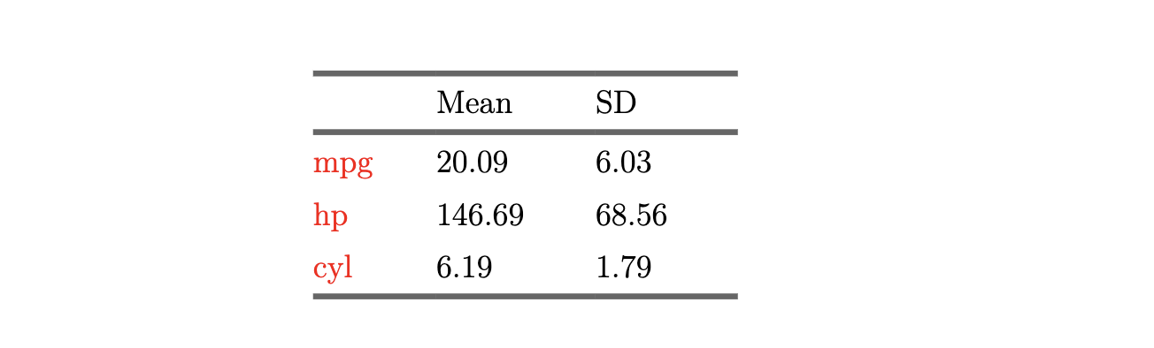
Summary statistics table
datasummary(
  mpg + hp + cyl ~ Mean + SD,
  data = mtcars,
  #--- add the title (caption) here ---#
  title = "Summary Statistics"
)
This is how the table would appear on the output PDF file.
7.7.1.3 Further modifying regression and summary statistics tables
You can modify (fine-tune) the output of modelsummary or gtsummary using the huxtable package if you are not satisfied. For the modelsummary package, this can be done by using output = "huxtable" and then use huxtable functions for modifications. Here is an example code.
modelsummary(list(lm_1, lm_2, lm_3),
 output = "huxtable",
 gof_omit = "IC|Log|Adj|F|Pseudo|Within",
 title = "Regression Results",
 stars = TRUE
) %>%
# Bold the header row
# set_bold(row = 1) %>%
# Border at the bottom of the table
set_bottom_border(row = nrow(.), value = 0.4) %>%
# Center-align the header
set_align(1, everywhere, value = "center") %>%
# Set font size to 10
set_font_size(value = 10)
For the gtsummary package, you can apply as_hux_table() and then modify the table.
Here is an example code for using the kableExtra package.
modelsummary(list(lm_1, lm_2, lm_3),
  output = "kableExtra",
  gof_omit = "IC|Log|Adj|F|Pseudo|Within",
  title = "Regression Results",
  stars = TRUE
) %>%
  kableExtra::add_header_above(
    c(" " = 1, "Model (se not clustered) " = 2, "Model (se clustered)" = 1)
  )
7.8 Figures (Cross-referenced)
7.8.1 Figures created internally
You can create plots within an Rmarkdown file and display them in the output PDF file. Here are the steps.
Create a plot using R
Add an R code chunk like this:
```{r fig-sample, fig.cap = "Sample figure title"}
figure_sample
```figure_sampleis a plot (R object).fig.cap: "Sample figure title"addsSample figure titleas the caption of the figurefig-sampleis the R chunk label and also the figure id used for cross-referencing
- Use
\@ref(fig:fig-sample)(fig:appended by the R chunk label) in the rmd file to cross-reference the figure (figure numbering in the output PDF file is automatic).
The figure in the PDF will have Sample figure title as the figure title.
Rmarkdown-PDF Comparison: Visual Example
7.8.2 Importing pre-made figures
To incorporate pre-made images or figures into your Rmarkdown document, especially when they are not generated within the Rmarkdown itself, you can use the knitr::include_graphics() function.
You can use the knitr::include_graphics() function to insert your desired image.
```{r fig-your-label, fig.cap = "Your Figure Caption"}
knitr::include_graphics("path_to_your_image.png")
```
Imported figures can be cross-referenced just like figures generated within R, as demonstrated previously.
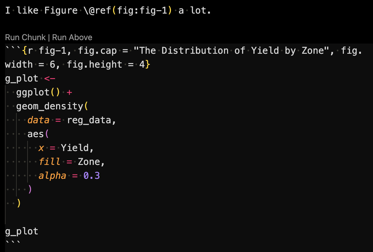
7.8.3 Figure placement and size
You can control the size of the plots in the output PDF file using the fig.width or fig.height option in the R code chunk. You can control the alignment of a figure using the fig.align. See an example below:
```{r fig-lable, fig.cap = "Title", fig.width = 6, fig.height = 4}
figure_sample
```
7.9 Mathematical Equations
7.9.1 Basics
You can fully take advantage of Latex math typesetting capability unlike the Rmarkdown-WORD system. This is because whatever you type inside of the following will be printed as is in the tex file when rmd file is converted to a tex file.
```{=tex}
whatever you type
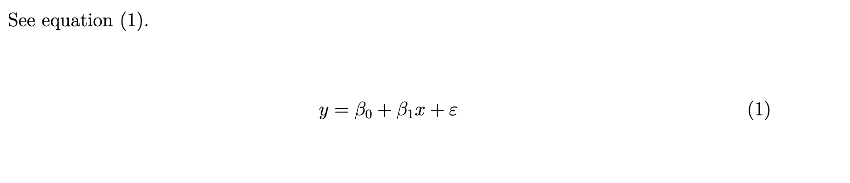
```So, for example, if you have the following in your rmd file,
```{=tex}
\begin{equation}
y = \beta_0 + \beta_1 x + \varepsilon
\end{equation}
```
then you will the following printed in the tex file,
\begin{equation}
y = \beta_0 + \beta_1 x + \varepsilon
\end{equation}
, which will then appear as
\[\begin{equation} y = \beta_0 + \beta_1 x + \varepsilon \end{equation}\]in the compiled pdf file.
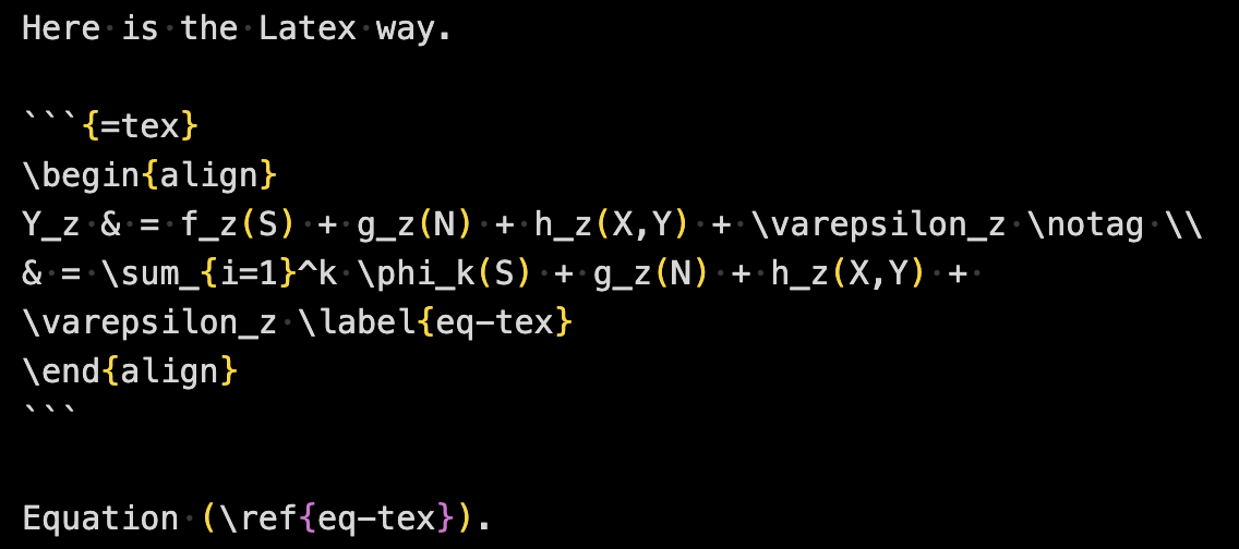
Of course, you can use other environments like align,
```{=tex}
\begin{align}
Y_z & = f_z(S) + g_z(N) + h_z(X,Y) + \varepsilon_z\notag \\
& = \sum_{i=1}^k \phi_k(S) + g_z(N) + h_z(X,Y) + \varepsilon_z
\end{align}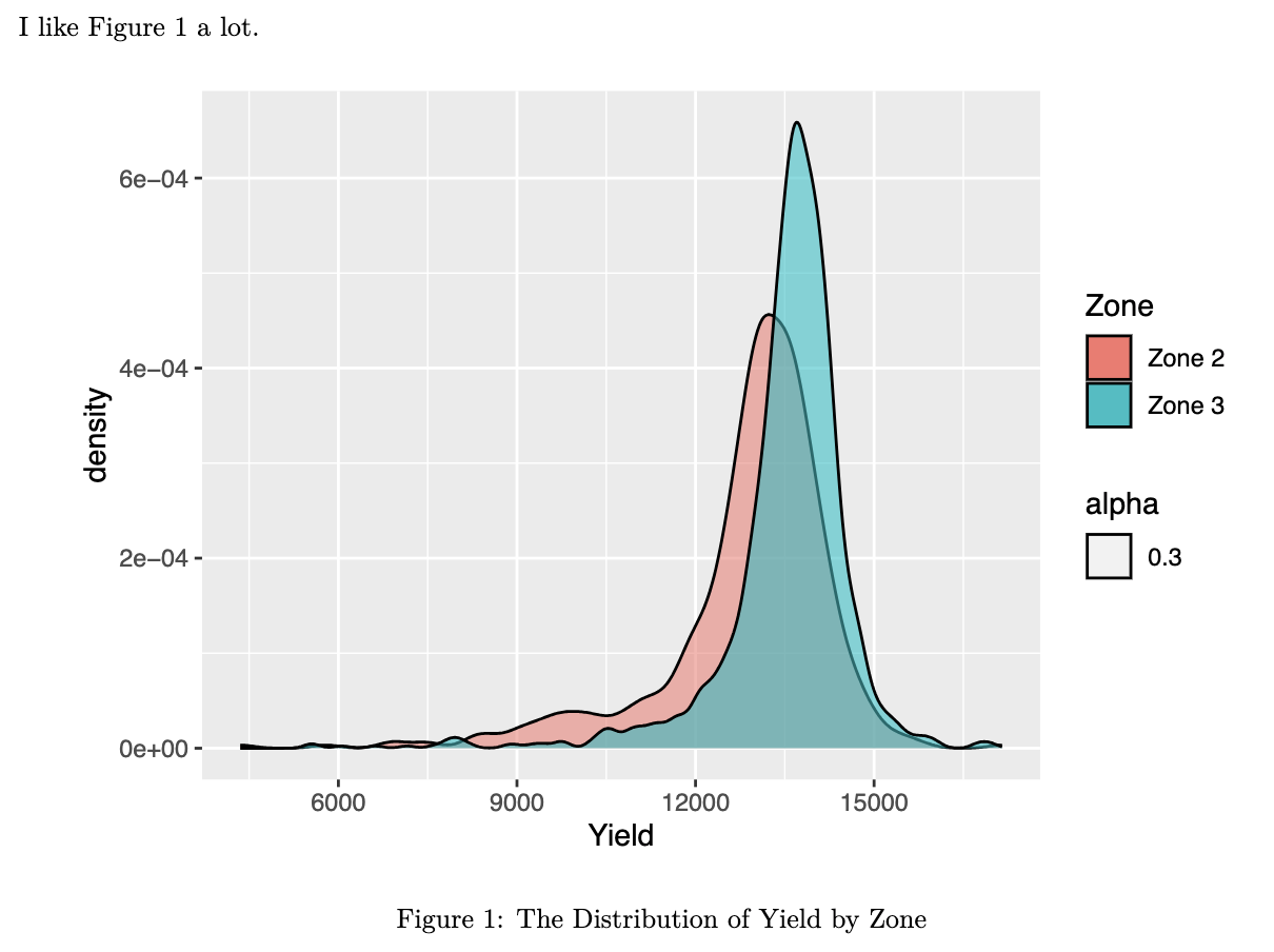
```7.9.2 Cross-reference
There are two ways to cross-reference equations. The first option is to place (\#eq:equation-name) at the end of the line that you would like to cross-reference. For example, (\#eq:eqn1) is placed at the end of the equation below.
```{=tex}
\begin{equation}
y = \beta_0 + \beta_1 x + \varepsilon (\#eq:eqn1)
\end{equation}
```
You can then write \@ref(eq:eqn1) to refer to the equation number.
Rmarkdown-Latex Comparison: Visual Example
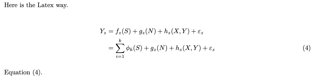
Alternatively, you can do cross-reference as if you would do in a tex file. Specifically, you can add \label{equation-name} at the end of the line and then write \ref{equation-name}.
```{=tex}
\begin{equation}
y = \beta_0 + \beta_1 x + \varepsilon \label{eq-tex}
\end{equation}
```
Rmarkdown-Latex Comparison: Visual Example
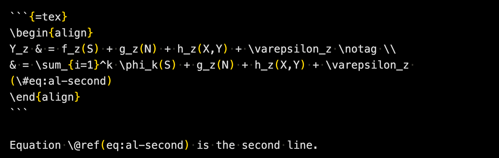
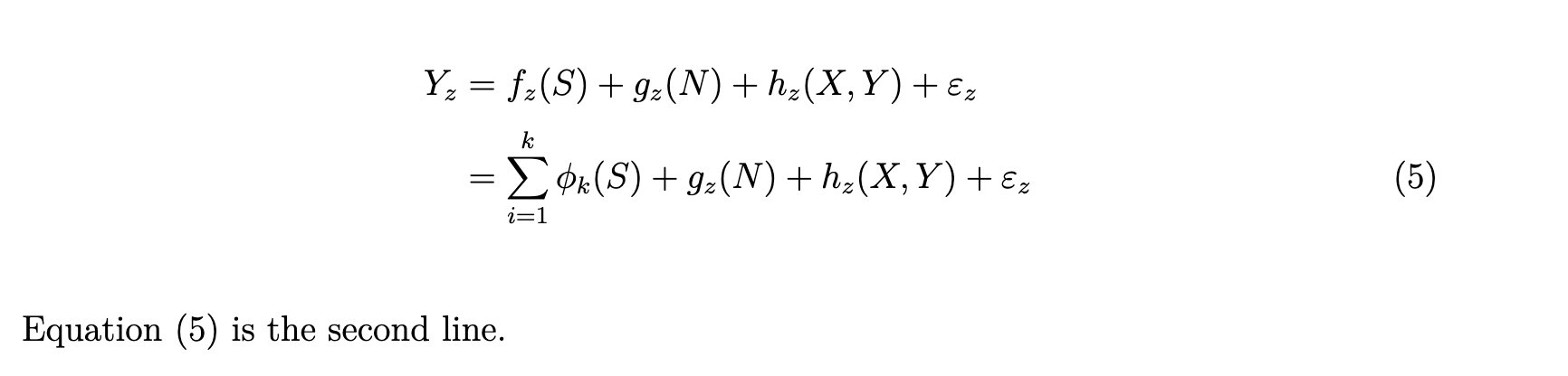
Just like Latex, you can use \notag to suppress equation numbers. You can cross-reference individual lines.
```{=tex}
\begin{align}
Y_z & = f_z(S) + g_z(N) + h_z(X,Y) + \varepsilon_z \notag \\
& = \sum_{i=1}^k \phi_k(S) + g_z(N) + h_z(X,Y) + \varepsilon_z (\#eq:al-second)
\end{align}
```

Equation \@ref(eq:al-second) is the second line.
Rmarkdown-Latex Comparison: Visual Example
7.10 Misccelaneous
7.10.1 Section number
Sometimes, you would like to have no section number for some of the sections. You can suppress section numbers by adding either {-} or {.unnumbered} at the end of the section title like below.
# Tables {-}7.10.2 Appendix
In order to have Appendix separate from the main narrative, you can start it by adding # (APPENDIX) Appendix {-} in the rmd file. Then the rest of the paper is considered a part of the Appendix section of the paper. By default, when you start a new section using #, then capitalized alphabets are used as the section indicator.
For example,
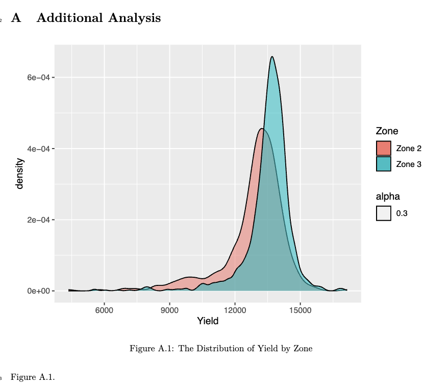
# (APPENDIX) Appendix {-}

# Additional Analysis
would translate into the following in the output pdf file.
Note that Appendix is not printed.
Confirm this by comparing sample_to_pdf.rmd and sample_to_pdf.pdf.
7.10.3 Figure numbering for Appendix
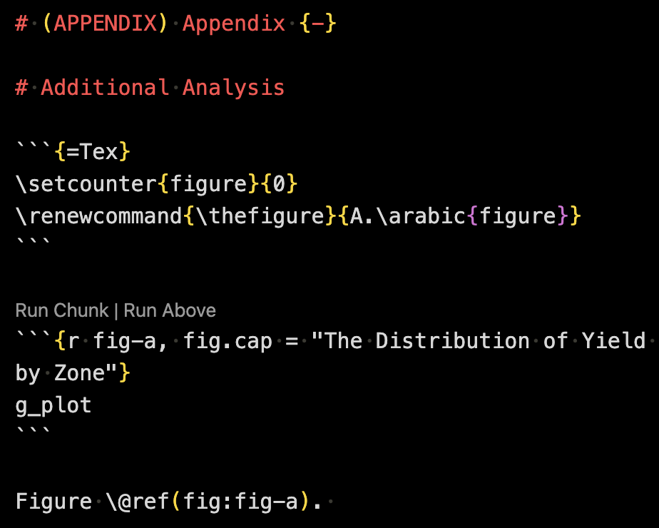
Since you can include Latex code to an Rmarkdown file, you can include Latex codes to achieve figure numbering that is separate from the main narrative. For example, the following code will add A. before figure number.
```{=Tex}
\setcounter{figure}{0}
\renewcommand{\thefigure}{A.\arabic{figure}}
```