R as GIS: Interaction of Vector and Raster Datasets
Before you start
Learning objectives
Learn the spatial interactions of a vector and raster dataset. Specifically,
Crop (spatially subset) a raster dataset based on the geographic extent of a vector dataset.
Extract values from raster data for points and polygons.
Table of contents
Pre-requisite (Links)
Tips to make the most of the lecture notes
Interactive navigation tools
Click on the three horizontally stacked lines at the bottom left corner of the slide, then you will see table of contents, and you can jump to the section you want
Hit letter “o” on your keyboard and you will have a panel view of all the slides
Running and writing codes
- The box area with a hint of blue as the background color is where you can write code (hereafter referred to as the “code area”).
- Hit the “Run Code” button to execute all the code inside the code area.
- You can evaluate (run) code selectively by highlighting the parts you want to run and hitting Command + Enter for Mac (Ctrl + Enter for Windows).
- If you want to run the codes on your computer, you can first click on the icon with two sheets of paper stacked on top of each other (top right corner of the code chunk), which copies the code in the code area. You can then paste it onto your computer.
- You can click on the reload button (top right corner of the code chunk, left to the copy button) to revert back to the original code.
Cropping and masking raster data
You have run on-farm nitrogen randomized experiment on a field to quantify the impact of nitrogen on corn yield.
You have three datasets
corn_yield:sfof corn yield (bu/acre) observations data represented by pointstreatment_blocks:sfof treatment blocks represented by polygonsNDRE:SpatRasterof NDRE (roughly put, an indicator of how green the field is) taken by a drone
Here is what they look like on a map:
Objective 1
Crop the NDRE raster data (NDRE) to the bounding box of corn_yield
We can create a map that is more focused on the area of interest rather than the entire field
We can stop carrying around the unnecessary parts of the data, which would educe its size (This matters when your raster data is spatially very fine and large.)
Extracting value to an
sffrom a smaller raster data is faster (we will talk about this later in this section)
Objective 2
Mask the NDRE data to treatment_blocks (assign NA to all the cells that are not intersecting with corn_yield)
- We can create a map without any unnecessary cells presented
You can crop a raster layer by using terra::crop().
Syntax
The resulting SpatRaster object is the original cropped to the bounding box of the sf object.
If you run the code above, then you should see an error. This happened because they do not share the same CRS.
Important!
- Projecting (or re-projecting to a different CRS) a raster dataset is typically a bad idea as it is irreversible.
- Re-project the vector data to the CRS of the raster data.
Let’s change the CRS of corn_yield to that of NDRE and then try to crop again.
Let’s check visually.
Syntax
The resulting SpatRaster object will have NA assigned to all the cells that are not intersecting with any of the geometries in the sf object.
Let’s check visually.
Note
- adding
na.value = "transparent"inscale_fill_*()will make the cells with NA value transparent (cannot be seen). - remove
na.value = "transparent"and run the code again, you will that cells with NA are grey.
We use
prism_us: a coarser version of PRISM precipitation data on 08/01/2012 covering the entire contiguous U.S. (SpatRaster)ne_counties: counties in Nebraska (sf)
Here is what they look like:
Create the map you saw in the previous tab.
Answer
Crop and then mask prism_us using ne_counties.
Create a map using the cropped- and masked-prism_us and ne_counties.
Answer
Extract values from raster layers to a vector data
Definition
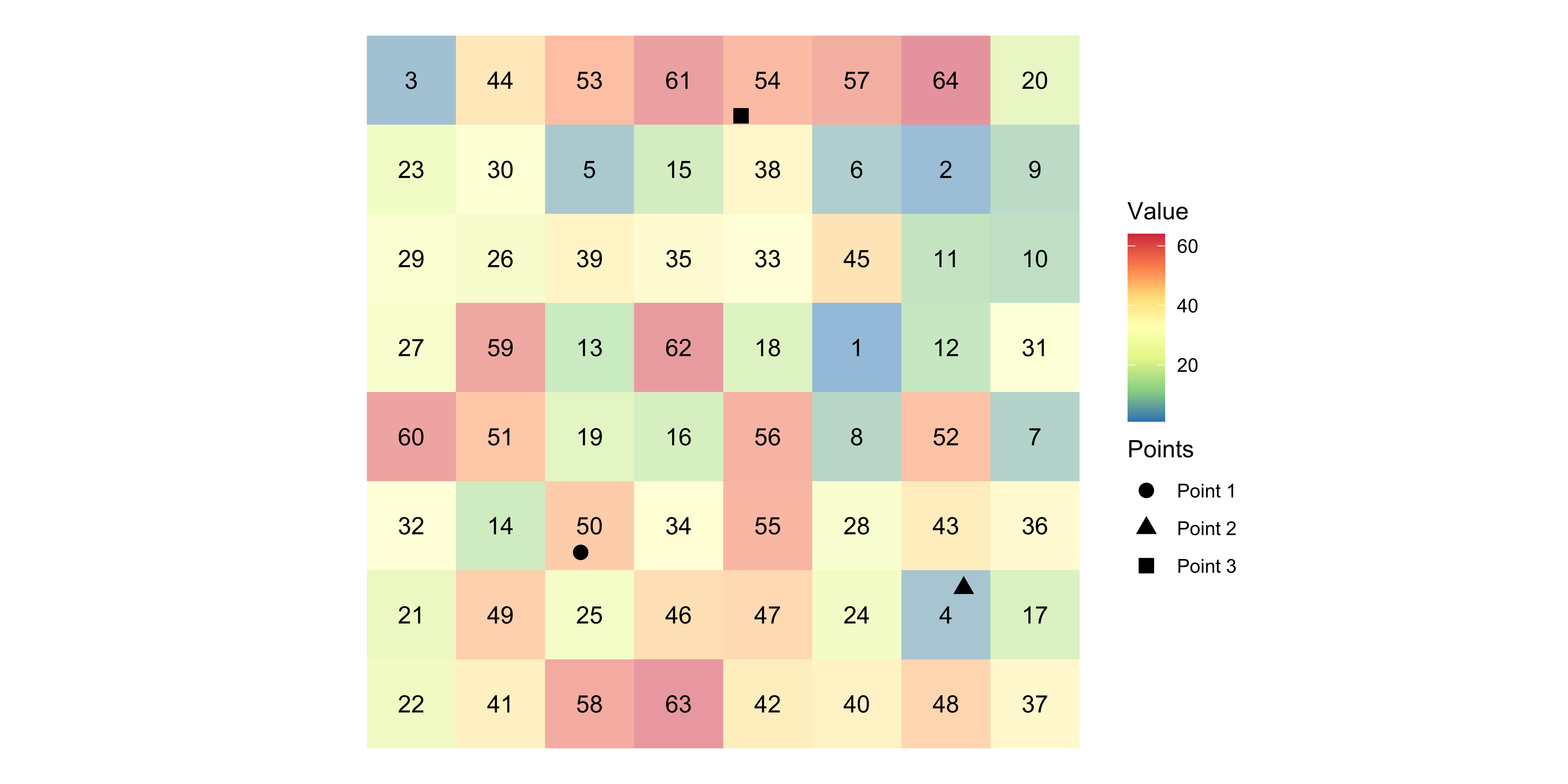
For each of the points, find which raster cell it is located within, and assign the value of the cell to the point.
Example

The numbers inside the cells are the values that the cells hold.
After the extraction,
- Point 1 will be assigned \(50\)
- Point 2 will be assigned \(4\)
- Point 3 will be assigned \(54\).
Definition
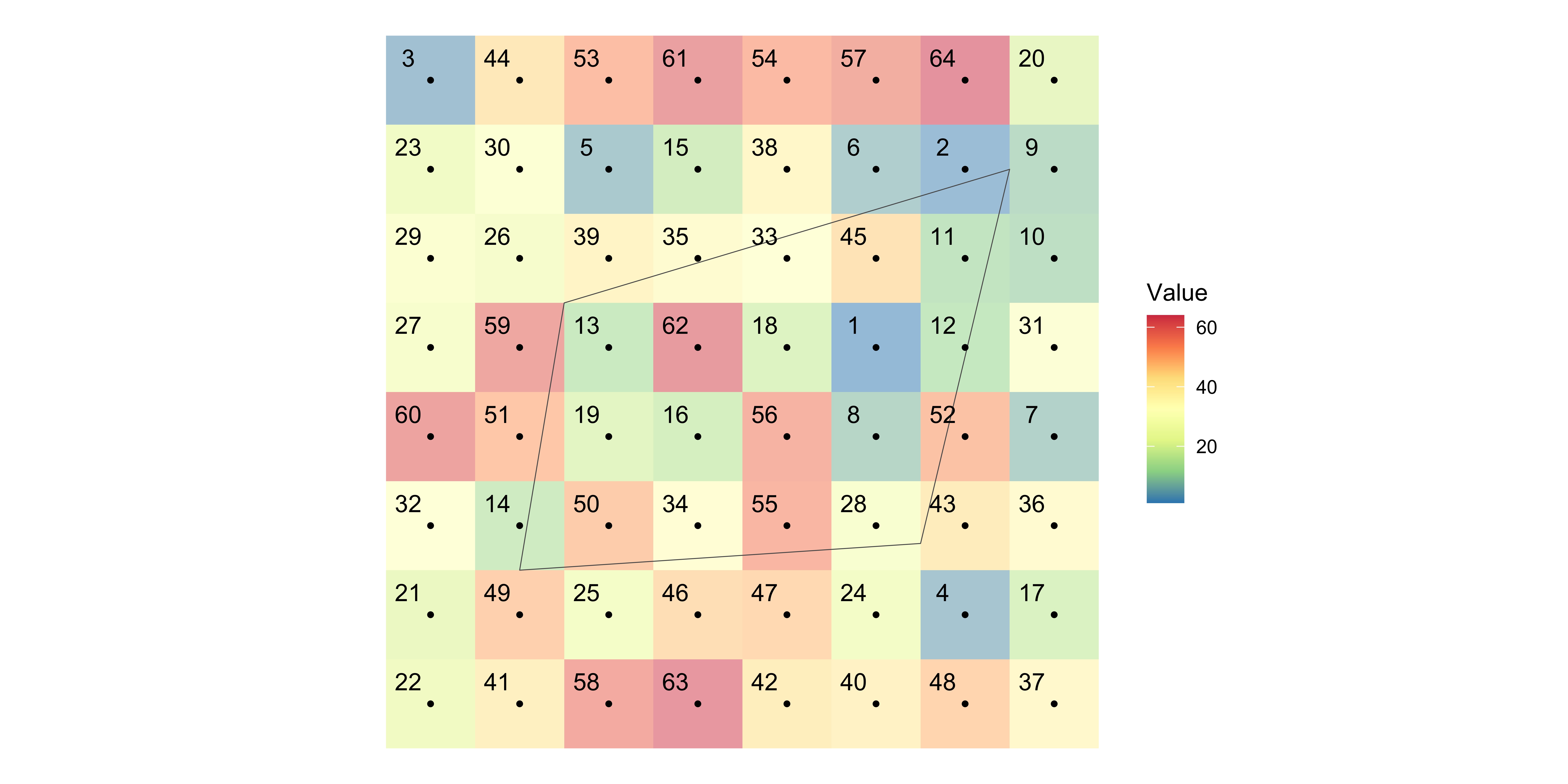
For each of the polygons, identify all the raster cells that intersect with the polygon, and assign a vector of the cell values to the polygon.
Example

Find all the raster cells each of the polygons “intersect with”
Assign the value of all the intersecting cells to the polygon (n-to-1).
Right now, corn yields (
corn_yield), NDRE (NDRE), and treatment blocks (treatment_blocks) are separate R objects.We would like to conduct two kinds of analysis
- analysis based on data where yield points are the unit of observations
- analysis based on data where treatment blocks are the unit of observations
To achieve this, we would like to
jointhem based on their locations- extract values from ‘NDRE’ to
corn_yield - extract values from ‘NDRE’ to
treatment_blocks
- extract values from ‘NDRE’ to
You can use terra::extract() with the following syntax.
Syntax
Extract NDRE values to each of the yield points:
Oops, we did it again.
Imporatant
IDvariable represents the row number in thesf(here,corn_yield). For example,ID == 3inNDRE_extractedis forcorn_yield[3, ].- This becomes more important when we we do extraction for polygons
Just extracting the raster values to the points is not where we stop.
We need to merge the extracted values back to the points data so that we can use them for further analysis.
Let’s first check the class of NDRE_extracted.
The nth row in NDRE_extracted is for the nth point in yield.
So, you can simply do this:
You can extract values from multiple layers at the same time using terra::extract() just like you did with a single-layer raster data.
For demonstration, let’s create a multi-layer raster data:
The resulting object is a data.frame and the values from first (second) layer is the second (third) column.
- How
- Demonstration
- Post-extraction processing
- Extract and summarize
- Area-weighted summarization
- Multiple layers
You can use terra::extract() with the following syntax. Yes, same as value extraction to points.
Syntax
Extract NDRE values to each of the treatment blocks:
It’s a data.frame.
As you can see below, there are more than one NDRE values for each of the treatment blocks, which is expected as there are many grid cells that are inside of them.
Let’s check the class of NDRE_extracted_tb.
We just want to one NDRE value for each of the treatment blocks. So, let’s summarize them. In doing so, we summarize by ID as it indicates the row number of treatment_blocks. Here, we are getting the average.
Now, we can assign the average NDRE values to treatment_blocks like below because ID == n is for nth row of treatment_blocks.
You can actually extract and summarize both in terra::extract() using the fun option.
In the previous cases of extraction and summarization tasks, all the intersecting cells are given the same weight irrespective of the degree of spatial overlap.
This is very much acceptable in the current application, because the resolution of the raster data is high (cells are so small) relative to the size of the polygons.
However, if the cells are relatively large, you might want to consider calculating area-weighted summary.
We can add exact = TRUE option, which returns fraction variable indicating the fraction of the cells intersecting with the polygon.
Just like the case with value extraction to points, we can extract values from multiple layers to polygons in a single call with terra::extract().
Let’s get the weighted average for both variables: