09-6: R as GIS: Download Spatial Datasets using R
U.S. county and state boundary
Transcript
County and state boundaries are the most reused spatial data in applied economics, since almost every administrative dataset is reported by county. The tigris package fetches them straight from the Census Bureau. It does far more than boundaries too, offering roads, water, tracts, block groups and a good deal else, so the link is worth following when you need something specific. The important thing is that a boundary file becomes one line of code rather than a download, an unzip, and a folder you have to remember the location of.
U.S. county and state boundary data are commonly used in many scientific studies.
The
tigrispackage is one of the packages that let you download them from within R.It lets you download much more than just county and state boundaries. See the other types of data here
Transcript
One function call. But look closely at the cb argument, because it matters more than it looks. Without it you get the full-detail boundary, which is very large and slow to draw, since it traces every inlet and river bend. With cb set to TRUE you get a generalised version, and for almost any map you will make, that is the right choice. Full detail is worth its cost only if you are doing precise spatial operations near a coastline. Note also progress bar set to FALSE, which just quiets the output.
The namespace in tigris colon-colon states means you can call the function without attaching the whole package. The assignment saves the returned sf object as states underscore s-f, so it contains state attributes together with the geometry needed for mapping. The second code block passes that object to ggplot, geom s-f draws its state polygons, and theme void removes axes and background decoration that do not help on a boundary map. The result beneath the code is your quick visual check that the download succeeded and the generalized state shapes are ready to use.
You can use
tigris::states()to download the state boundary data as ansfobject.By default, the most detailed boundary data is downloaded, which can be quite large
- creating map using
ggplot()can take significantly more time - the map can be quite large in size
- creating map using
By adding
cb = TRUE, you will get generalized (less detailed) boundary data, which is usually sufficient.

Transcript
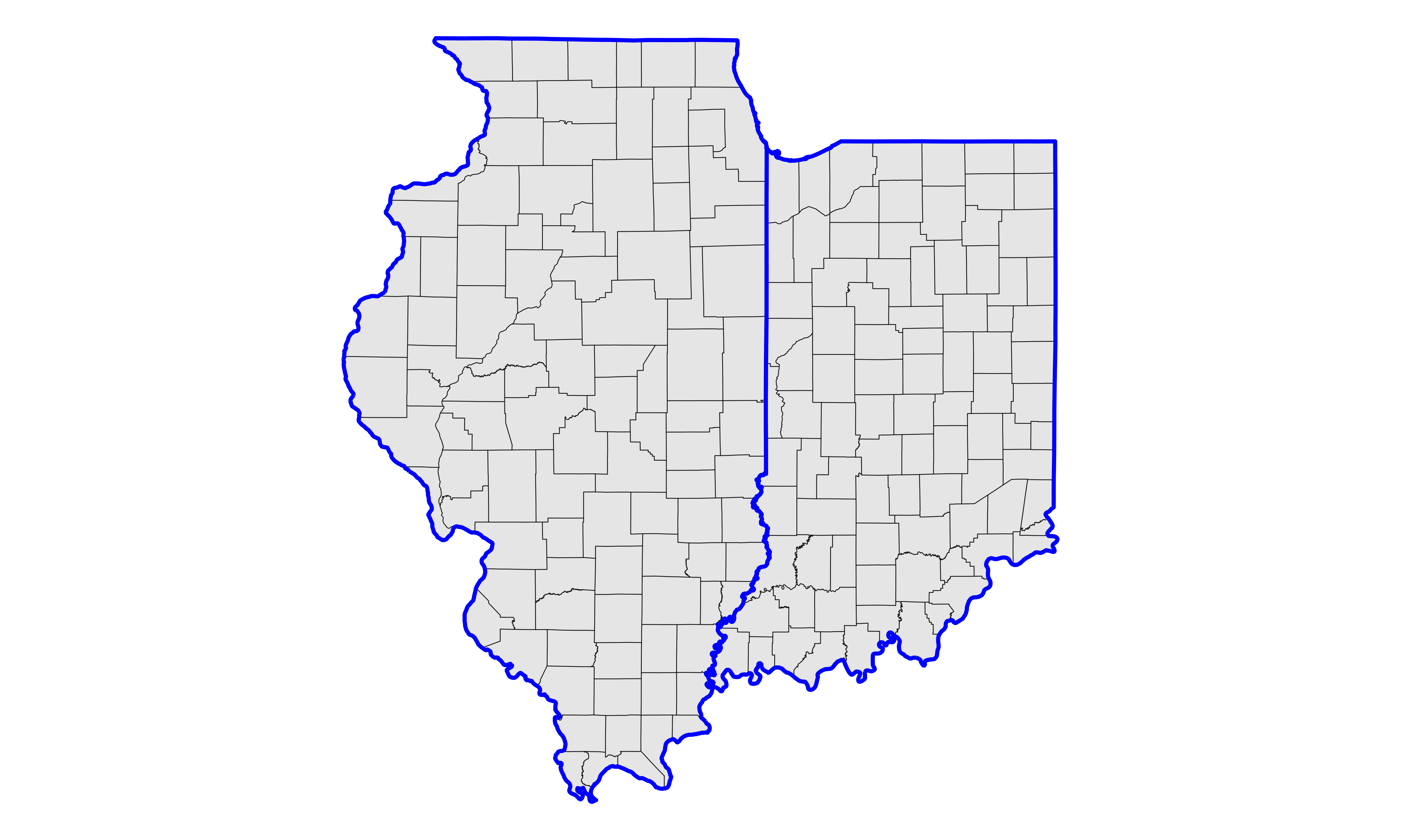
The counties function works the same way, with a state argument that takes abbreviations or names and accepts several at once. The map at the end is worth a moment: county boundaries drawn underneath, then the two state outlines over the top in blue and thicker. That is the layering from the mapping deck used for something practical, checking that two datasets you downloaded separately actually line up. If the state outlines had not sat exactly on the county edges, you would know something was wrong immediately, usually because the boundary vintages differ or the CRS metadata is incorrect or missing.
Here the state argument receives a vector containing Illinois and Indiana, cb asks for generalized county boundaries, and progress bar false keeps the download quiet. The result is stored as I-L underscore I-N underscore county. In the map, the empty ggplot call is useful because each geometry layer supplies its own data. The first geom s-f draws every downloaded county. The second filters the earlier state object so the name is Illinois or Indiana, sets fill to N-A so those polygons stay transparent, and uses blue with linewidth one to make only their outer borders prominent. Theme void then removes the non-map furniture.
You can use
tigris::counties()to download the county boundary data as ansfobject.You can specify states by the
stateoption.
PRISM
Transcript
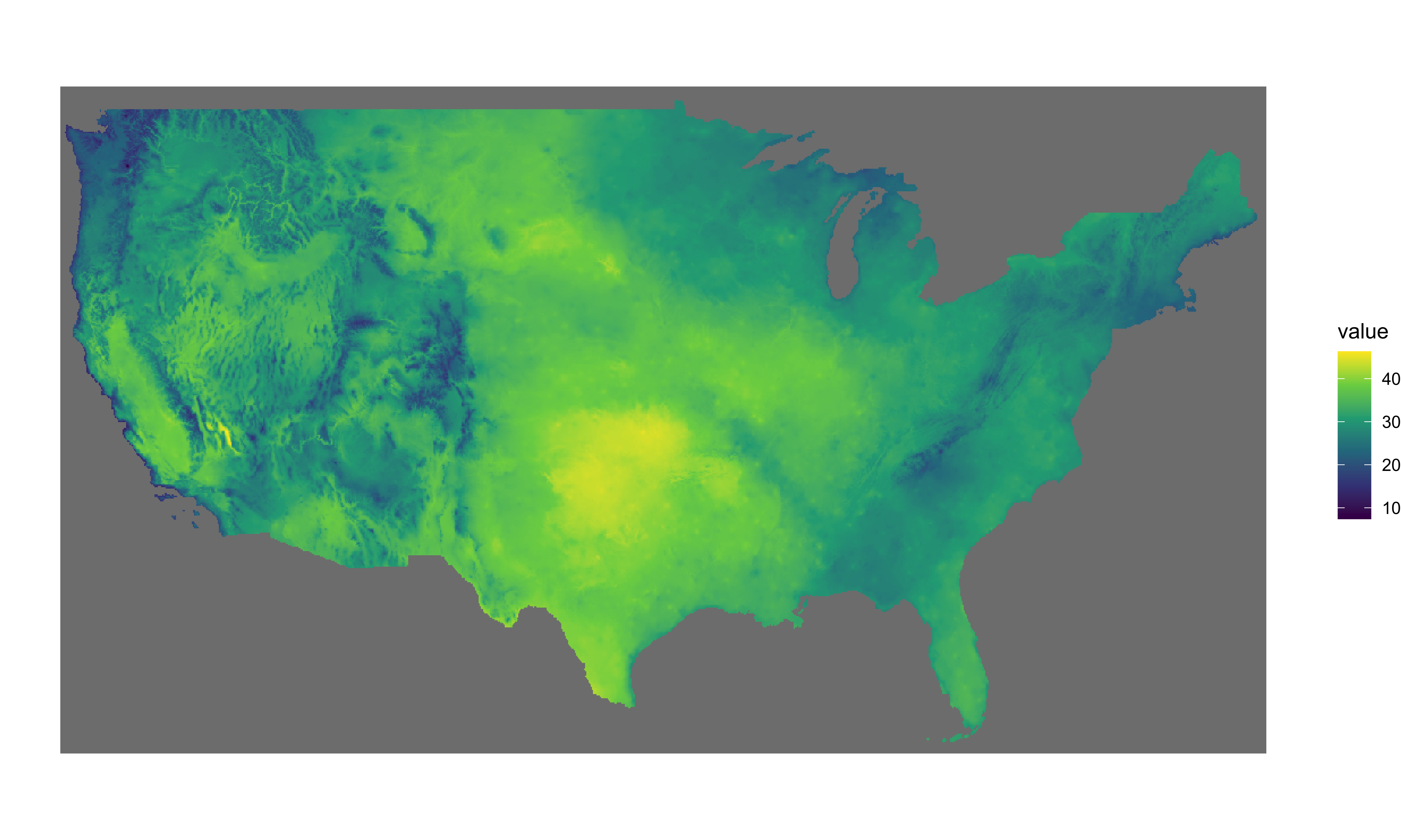
PRISM is the standard source for United States weather in applied work: daily precipitation and maximum and minimum temperature, modelled onto a four kilometre grid covering the whole country. It is raster data, so everything from the raster deck applies, and the map on this slide is a single day of maximum temperature. If you need weather as a control variable, or you are estimating anything at all about climate and agriculture, this is very likely where your data will come from. It is free, and it covers several decades at daily resolution.
The source description also includes daily mean temperature, alongside precipitation and minimum and maximum temperature. The displayed example reads the BIL raster for maximum temperature on August first, 2012. Geom spatraster draws the grid cells, the continuous viridis fill scale turns their values into an ordered color gradient, and theme void removes axes and background elements so the spatial temperature pattern is the focus. This output is also a reminder that a PRISM download is not a table with one row per county. It is a surface made of cells, which is why you read and process it with terra.
The PRISM dataset provides model-based estimates of daily precipitation, maximum temperature, and minimum temperature for the U.S. at the 4km by 4km spatial resolution.
Transcript
One function fetches a date range, and the four arguments are all it takes. Type is the variable, using the abbreviations listed. The two dates bound the range, in year-month-day order. And keepZip decides whether the compressed downloads are kept after unpacking, which you usually do not want. Read the note about setting the download directory first, and note the modern spelling of it, since older code you find online will use an options call instead. Both do the same job, but the function is the current spelling and is easier to remember.
You can use get_prism_dailys() from the prism package to download PRISM data.
Syntax
type: you can select from “ppt” (precipitation), “tmean” (mean temperature), “tmin” (minimum temperature), and “tmax” (maximum temperature).minDate: starting date specified in format YYYY-MM-DDmaxDate: end date specified in format YYYY-MM-DDkeepZip: ifFALSE, the zipped folders of the downloaded files will not be kept; otherwise, they will be kept.
Before you download PRISM data, set the folder the files should be stored in:
Transcript
This one you genuinely have to run yourself, since it writes files to disk. Five days of precipitation is enough to see the shape of the thing. Pay attention to what you end up with, because it is the reason the next tab exists: one folder per day, each holding several files that share a name and differ only by extension. That is the BIL format from the raster deck, where the values, the header describing the grid, and the projection information all live in separate files that have to stay together in the same folder.
The first block attaches prism and sets lectures slash Data slash PRISM as the download directory. Change that path to a location on your own computer before running it. The second block asks get_prism_dailys for ppt, the package abbreviation for precipitation, from January first through January fifth of 2024. KeepZip false tells prism not to retain the downloaded zip archives after unpacking them, so you keep the usable files without duplicate compressed copies. These chunks have evaluation turned off in the deck because the download needs a normal local R session and a real place to write the folders.
First set the path:
Now, download:
This will create a single folder for each day of the specified date range. Inside each folder you will see a bunch of files sharing one name and differing only in extension.
Transcript
The practical problem: a year of daily data is three hundred and sixty-five folders, and you are not going to type those paths. So list them programmatically. The code recurses through the folder, uses an end-anchored pattern to keep only paths ending in bil, and drops the auxiliary ones, which would otherwise sneak in. Then terra reads the whole vector in a single call and gives you one multi-layer object with a layer per day. That last step is the one worth remembering: terra’s rast function accepts a whole vector of paths, not just a single one, and stacks them for you.
Read the pipeline from left to right. List files starts at Data slash PRISM. Recursive true searches the daily subfolders, and full names true returns complete paths relative to that starting point so rast can locate each file. In the first grep, backslash-dot means a literal period and the dollar sign anchors bil at the end; value true keeps the matching paths instead of their positions. The next line uses grepl to mark names containing aux, the exclamation mark reverses that test, and the bracket keeps only the non-auxiliary files. The parentheses around the assignment print the resulting path vector for inspection. Replace the starting folder with your own, then pass the checked vector to terra colon-colon rast as shown.
As you have seen, we would have many files to open unless the specified date range is very short. Rather than naming them one by one, list them programmatically.
First, the following code gives you the names of all the PRISM files with the .bil extension.
(
  prism_files_list <-
    list.files("Data/PRISM", recursive = TRUE, full.names = TRUE) %>%
    grep(pattern = "\\.bil$", ., value = TRUE) %>%
    .[!grepl("aux", .)]
)
[1] "Data/PRISM/PRISM_ppt_provisional_4kmD2_20240101_bil/PRISM_ppt_provisional_4kmD2_20240101_bil.bil"
[2] "Data/PRISM/PRISM_ppt_provisional_4kmD2_20240102_bil/PRISM_ppt_provisional_4kmD2_20240102_bil.bil"
[3] "Data/PRISM/PRISM_ppt_provisional_4kmD2_20240103_bil/PRISM_ppt_provisional_4kmD2_20240103_bil.bil"
[4] "Data/PRISM/PRISM_ppt_provisional_4kmD2_20240104_bil/PRISM_ppt_provisional_4kmD2_20240104_bil.bil"
[5] "Data/PRISM/PRISM_ppt_provisional_4kmD2_20240105_bil/PRISM_ppt_provisional_4kmD2_20240105_bil.bil"
[6] "Data/PRISM/PRISM_tmax_stable_4kmD2_20120801_bil/PRISM_tmax_stable_4kmD2_20120801_bil.bil"
[7] "Data/PRISM/tmax/PRISM_tmax_stable_4kmD2_20230601_bil/PRISM_tmax_stable_4kmD2_20230601_bil.bil"
[8] "Data/PRISM/tmax/PRISM_tmax_stable_4kmD2_20230602_bil/PRISM_tmax_stable_4kmD2_20230602_bil.bil"
[9] "Data/PRISM/tmax/PRISM_tmax_stable_4kmD2_20230603_bil/PRISM_tmax_stable_4kmD2_20230603_bil.bil" Just replace "Data/PRISM" with your folder path to the PRISM files.
We can now read them using terra::rast() like below:
class       : SpatRaster
size        : 621, 1405, 9  (nrow, ncol, nlyr)
resolution  : 0.04166667, 0.04166667  (x, y)
extent      : -125.0208, -66.47917, 24.0625, 49.9375  (xmin, xmax, ymin, ymax)
coord. ref. : lon/lat NAD83
sources     : PRISM_ppt_provisional_4kmD2_20240101_bil.bil
              PRISM_ppt_provisional_4kmD2_20240102_bil.bil
              PRISM_ppt_provisional_4kmD2_20240103_bil.bil
              ... and 6 more sources
names       : PRISM~1_bil, PRISM~2_bil, PRISM~3_bil, PRISM~4_bil, PRISM~5_bil, PRISM~1_bil, ...
min values  :       0.000,      0.0000,      0.0000,      0.0000,      0.0000,       7.408, ...
max values  :      42.917,     10.2093,     87.7497,     37.0813,     90.0984,      46.303, ...
Transcript
The same three-step arc as the NASS exercise, now for weather: download three days of maximum temperature, read them all back with the listing trick, and facet a map by layer. Note the third answer uses facet_wrap on lyr, which is the raster faceting from the mapping deck. Worth noticing how little of this is new. By this point in the course you are combining pieces you already know rather than learning anything fresh, which is roughly the definition of having learned something. That is a fair note to end the course on.
In Download PRISM data, change the folder passed to prism_set_dl_dir, then request type tmax for June first through June third of 2023. KeepZip false discards the archives after extraction. In Read the downloaded files, list files searches that tmax folder recursively and returns full paths, the anchored bil filter keeps the raster data files, and the auxiliary-name filter removes unwanted companions. Terra rast reads the remaining vector into prism underscore max underscore temp, with one layer for each downloaded day.
In Create a map, geom spatraster draws that multi-layer object. Facet wrap with lyr makes a panel for each layer name, so the three daily temperature surfaces appear separately rather than being drawn on top of one another. As in the NASS exercise, the folded answers let you attempt each operation before revealing the working code.
Download PRISM maximum temperature data from “06-01-2023” to “06-03-2023”.
Answer
Read all the maximum temperature data files you just downloaded using terra::rast().
Answer
Crop Data Layer
Transcript
The Cropland Data Layer is a remarkable satellite-derived dataset. Coverage began on a limited basis in 1997 and expanded to the entire continental United States in 2008. Its resolution is thirty metres from 2008 through 2023 and ten metres from 2024 onward, classifying pixels by what crop is growing on them. For agricultural economics it is close to indispensable, since it tells you what was actually growing on a given field rather than what somebody reported at the county level. CropScape is the interactive front end you may have seen in a browser, and the CropScapeR package talks to exactly the same service from R, which is what we use here.
The resolution history on screen also includes fifty-six metres in 2006 and 2007, before the move to thirty metres in 2008. This is a georeferenced, crop-specific land-cover product from USDA NASS, so each raster cell records a land-cover class at a known location. That cell-level detail is the reason the dataset supports field-scale and landscape analysis that county summaries cannot. The CropScape link is useful for exploring the product visually, while the package workflow makes the same kind of request reproducible in a script.
The Cropland Data Layer (CDL) is a data product produced by the National Agricultural Statistics Service of U.S. Department of Agriculture.
CDL provides geo-referenced, high-accuracy, crop-specific cropland land cover information. Coverage began on a limited basis in 1997 and expanded to the entire continental United States in 2008. Resolution was 56 meters in 2006 and 2007, 30 meters from 2008 through 2023, and 10 meters from 2024 onward.
This data product has been extensively used in agricultural research. CropScape is an interactive Web CDL exploring system, and it was developed to query, visualize, disseminate, and analyze CDL data geospatially through standard geospatial web services in a publicly accessible on-line environment (Han et al., 2012).
This section shows how to use the CropScapeR package (Chen 2020) to download and explore the CDL data.
Transcript
The package offers four functions, but one of them does the work. GetCDLData downloads the raw layer. The other three create preview images, summary statistics, and between-year change comparisons. Learn that one properly and treat the other three as a bonus you may never need. One thing to note before you go looking for it: what comes back is a RasterLayer from the old raster package, not a terra SpatRaster, so you will usually pass it straight through terra’s rast function to convert it, exactly as the final exercise does.
The package implements some of the most useful geospatial processing services provided by the CropScape, and it allows users to efficiently process the CDL data within the R environment.
Specifically, the CropScapeR package provides four functions that implement different kinds of geospatial processing services provided by the CropScape.
GetCDLData()in particular is the most important function as it lets you download the raw CDL data.The other functions provide the users with the CDL data summarized or transformed in particular manners that may suit the need of some users.
Transcript
Three arguments, and the fiddly one is type, which tells the service how to interpret the area you gave it. An f means you passed a FIPS code, for a state or a county. A b means a bounding box, and that includes handing it an sf object, since only the box gets used. A p is a single point and ps a polygon of your own coordinates. Read the callout about the class of the returned object too, because forgetting it produces confusing errors two steps later, when some terra function refuses what you hand it.
Aoi is the area you want covered, and year chooses the CDL vintage. Match the type to the form of that area. An sf or s-f-c object uses letter b, as does a bounding box defined by four corner points. A county uses its five-digit FIPS code with letter f, while a state uses its two-digit FIPS code with the same type. A polygon described by at least three coordinates uses p-s, and one coordinate uses p for a point. These are service codes, so choosing the wrong one changes how the server reads the same value. The result is a raster-package RasterLayer, as the callout emphasizes, so convert it before using a workflow that expects terra’s SpatRaster class.
GetCDLData() allows us to obtain CDL data for any Area of Interest (AOI) in a given year. It requires three parameters to make a valid data request:
aoi: Area of Interest (AOI).year: Year of the data to request.type: Type of AOI.
The following AOI-type combinations are accepted:
- any spatial object as an sf or sfc object -
type = "b" - county (defined by a 5-digit county FIPS code) -
type = "f" - state (defined by a 2-digit state FIPS code) -
type = "f" - bounding box (defined by four corner points) -
type = "b" - polygon area (defined by at least three coordinates) -
type = "ps" - single point (defined by a coordinate) -
type = "p"
Transcript
A whole state by FIPS code, Nebraska being thirty-one, with type set to f. The warning about time is not a formality. At thirty metre resolution a state contains an enormous number of cells, and the download and the memory it needs are both substantial. This is exactly why cropping matters, and why the next example takes four counties rather than a state. If you only need part of a state, ask for that part rather than downloading everything and throwing most of it away. Your patience and the server will both benefit.
The code stores the request as c-d-l underscore N-E. Aoi thirty-one identifies Nebraska, year is the character value 2018, and letter f tells the service to interpret thirty-one as a FIPS code rather than as a point or a box. Evaluation is turned off on the slide, so there is no displayed raster output and you must run the request locally if you need it. The object returned by this call is the RasterLayer class noted on the previous tab.
Suppose you are interested in getting CDL data for the entire Nebraska.
In this case we can use the state FIP code for NE (31) for
aoiand specifytypeto be"f"(Note that this would take some time if you run it.).This can take a while. Since the spatial resolution is 30m, the CDL data covering the whole of Nebraska has an enormous number of cells and is memory-intensive.
Transcript
The more typical case, and the more sensible one. Pull county boundaries with tigris, filter to the four you want, and hand that sf object straight to GetCDLData. Note what the service actually does with it, which is explained on the download tab: it uses only the bounding box, not the outlines, so you get a rectangle containing your counties along with the corners of their neighbours. Trimming that rectangle back to the actual county shapes is masking, from the previous deck, and it is one of the things the final exercise asks you to do.
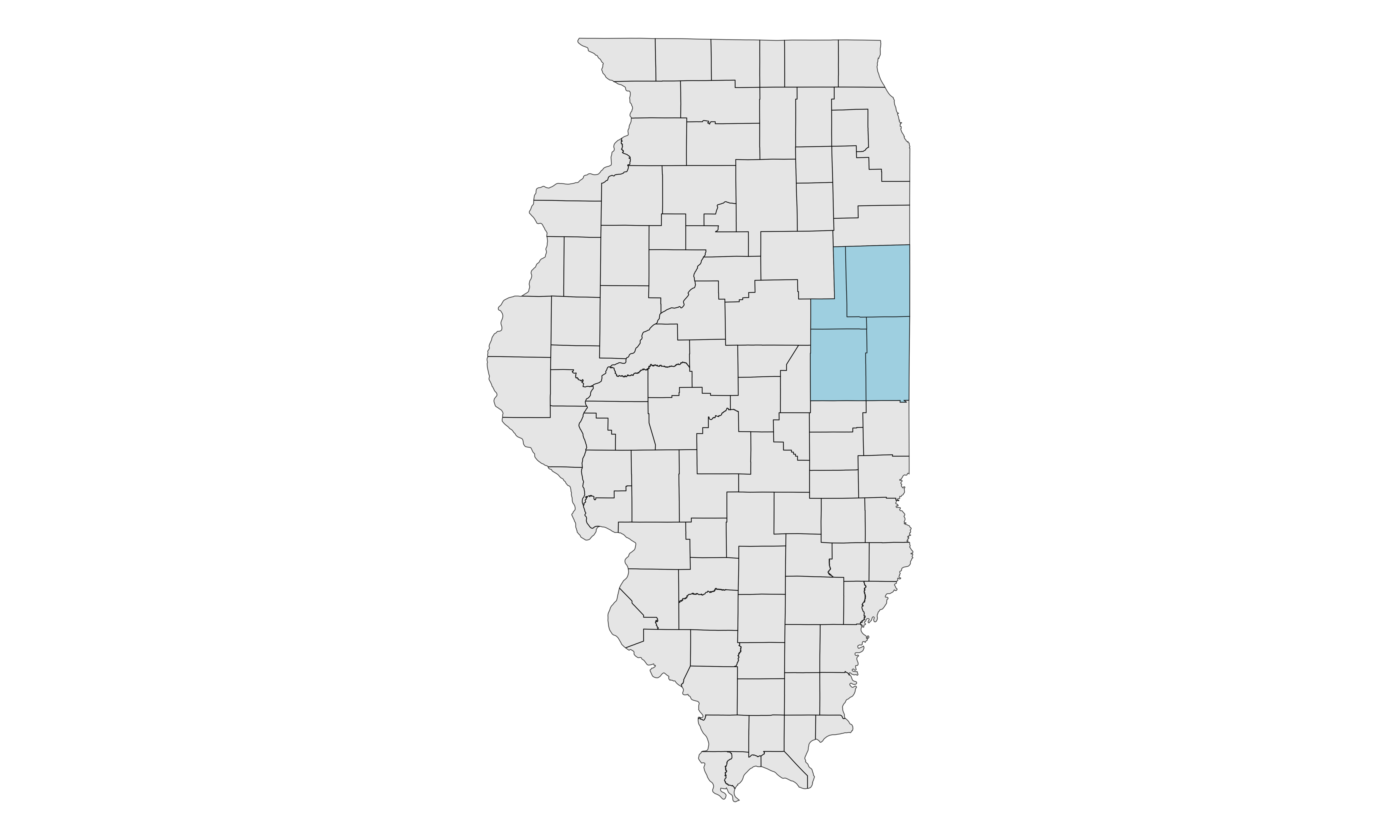
On Area of interest, tigris counties downloads Illinois with generalized boundaries and no progress display. The membership filter keeps Champaign, Vermilion, Ford, and Iroquois in I-L underscore four underscore county. The output map first draws every Illinois county, then overlays those four with light-blue fill; theme void strips away the axes. That picture is a visual check that the filter selected the intended connected area.
On Download, the sf object becomes aoi, the requested year is 2018, and type b tells GetCDLData to use its bounding box. Because the call is not assigned in the shown code, running it displays or returns the download but does not save a named object for later steps. In your own workflow, assign that result if you plan to convert, mask, or map it. The rectangular extent is efficient to request, but remember that it is not the same shape as the four county polygons.
In this example, we are interested in obtaining CDL data for the following four counties in Illinois: Champaign, Vermilion, Ford, and Iroquois.
Let’s first get the county boundary data for them:
Here is where they are:
Transcript
The final exercise of the course, and it pulls in nearly everything. Download a county boundary with tigris, use it to fetch CDL data, convert to a SpatRaster, mask it to the county outline, aggregate it to something a computer can plot, and map the result. That is four decks’ worth of material in five steps. One thing to watch in the aggregation: CDL cells hold crop codes rather than quantities, so averaging them is meaningless. Take the most common code in each block instead, with the modal function, exactly as the raster deck warned.
On AOI, tigris counties requests generalized Iowa county boundaries, and the pipe sends them directly to dplyr filter. The exact name test keeps Sioux County and stores the one-feature sf object as sioux underscore county. On Download, that object is the aoi, 2022 is the requested CDL year, and type b requests its bounding box. The pipe immediately passes the returned RasterLayer to terra rast, so sioux underscore c-d-l underscore 2022 is a SpatRaster ready for the remaining terra operations.
On Mask, the county boundary is first transformed to the raster’s coordinate reference system. That alignment is necessary because masking compares locations, and coordinates in different systems cannot be compared correctly. Terra mask then keeps cells inside Sioux County and removes cells in the rest of the downloaded rectangle. On Aggregate, fact ten groups the original cells into ten-by-ten blocks. Fun modal assigns each larger cell the most common crop code in its block, preserving the categorical meaning while reducing the number of cells that must be drawn.
Finally, ggplot starts the map and geom spatraster draws sioux underscore aggregated. The code-folded answers are there for checking, so work through the tabs in order before opening them. The object names deliberately carry forward from one answer to the next, which makes this a single reproducible pipeline from an administrative boundary to a manageable county land-cover map.
Using the tigris package, download the county boundary for Iowa, and then filter it to keep only the Sioux county. Name the sf file sioux_county.
Answer
Using the CropScapeR::GetCDLData(), download the 2022 CDL data covering the Sioux County. Then, convert it to a SpatRaster object. Name the final product sioux_cdl_2022.
Answer
Mask the CDL data you just downloaded using sioux_county using terra::mask().
Answer
Before creating a map from the downloaded CDL layer data, let’s aggregate the data by factor of 10 using terra::aggregate(). Call it sioux_aggregated.
Careful with fun here — CDL cells hold crop codes, not quantities.
Answer
Code
#--- CHANGED: fun = "modal" added. aggregate() defaults to fun = "mean", and ---#
#--- averaging land cover codes (1 = corn, 5 = soybeans, ...) produces       ---#
#--- numbers that are not any crop. "modal" takes the most common code in    ---#
#--- each block, which is the only sensible summary for a categorical layer. ---#
sioux_aggregated <- terra::aggregate(sioux_masked, fact = 10, fun = "modal")