Let us begin by being precise about the problem IV is meant to solve. The equation on screen says that the expected value of the error, conditional on all of the explanatory variables from x one through x k, is not zero. In other words, once you know the regressors, you can systematically predict something about the error. That violates the zero conditional mean assumption that gives OLS a causal interpretation.
The next definition focuses on one regressor. If x k is correlated with the error term, we call x k endogenous. The error contains every unobserved determinant of the outcome, so this correlation means that changes in x k come bundled with changes in something omitted from the regression. OLS cannot tell which part of the resulting outcome difference came from x k itself.
The four bullets list common routes to that failure. With an omitted variable, a factor left in the error affects both the regressor and the outcome. With selection, the observations or treatment status enter the sample through a process related to unobserved outcomes. With reverse causality, the outcome also helps determine the supposed cause. With measurement error, the observed regressor differs from the true regressor, and that discrepancy becomes part of the regression error. These mechanisms are different, but each can create correlation between a regressor and the structural error.
Instrumental variables do not somehow make the original regressor exogenous. Instead, IV looks for a separate source of variation that moves the endogenous regressor but is unrelated to the outcome error. We will use only that isolated variation to estimate the causal effect. The next tab draws the endogeneity problem as a causal diagram, which will make the source of the OLS failure visible.
Endogeneity
E[u\mid x_1,\dots,x_k]\ne0
The zero-conditional-mean assumption fails: the error term is systematically related to at least one explanatory variable.
Endogenous independent variable
If an explanatory variable x_k is correlated with the error term, we call x_k an endogenous explanatory variable.
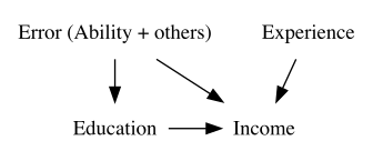
Here is the running example in a causal diagram. The two bullets above the figure identify the target: education is the explanatory variable whose causal effect we want, and income is the outcome. In the diagram, the arrow from Education to Income is therefore the causal relationship we would like to estimate.
Now trace every other arrow. Experience points to Income because labor-market experience can affect earnings, and it is an observed variable that we can include as a control. The box labeled Error contains ability plus other determinants that we have not observed or have not included separately. It points to Income because ability and those other factors affect earnings. Crucially, it also points to Education because ability, preferences, family circumstances, or similar omitted factors can influence how much schooling a person obtains.
That pair of arrows creates the backdoor path Education, Error, Income. People with different education levels will tend to differ in the omitted factors even before education has any causal effect. A regression of income on education and experience would then use two kinds of education variation at once: variation that might causally change income, and variation associated with ability and the other contents of the error. Controlling for experience blocks the path through experience if the specification is adequate, but it does not block the path through the unobserved Error node. Consequently, the education coefficient generally combines the causal effect with omitted-variable confounding.
The code shown above the figure is only how the diagram was generated. The substantive lesson is the arrow pattern. On the next tab we add a new variable, Z, and ask what arrows it may and may not have if it is to solve this problem.
You want to estimate the causal impact of education on income.
Causal diagram
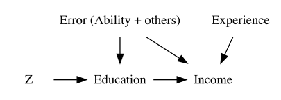
Now look at the new node Z on the left. We want Z to create a particular chain: Z changes Education, and Education in turn changes Income. The arrow from Z to Education represents relevance. In words, Z must predict education even after we control for the other exogenous variables, such as experience. If Z does not move education, it gives us no new education variation with which to learn the education effect.
The absence of arrows is just as important as the arrow we see. Exclusion means there is no direct arrow from Z to Income. After holding education and the included controls fixed, Z must not change income through any other channel. Exogeneity means Z is uncorrelated with the structural error, including ability. In a fuller diagram, there must be no unblocked common cause that makes Z vary with unobserved determinants of income.
If all three ideas hold, we can compare the part of education that changes because Z changes. That instrument-induced education variation travels to income through the causal arrow we care about, while avoiding the backdoor path through ability. Notice that experience still points to income, so it remains an included control. The instrument is not a substitute for correctly specifying the exogenous controls.
This picture also shows why a good prediction of education is necessary but insufficient. A variable could have a very strong Z-to-Education arrow and still be invalid if it directly affects income or shares an unobserved cause with income. Relevance is an empirical first-stage question. Exclusion and exogeneity are causal design claims. Keep those three concepts separate as we translate the diagram into two-stage least squares on the next tab.
We want to find a variable like Z in the diagram below:
The model at the top is the structural outcome equation. Y is the outcome. Beta zero is the intercept. Beta one is the causal coefficient on x one, the variable of interest. Beta two is the coefficient on x two, an included control. U collects all unobserved determinants of y.
The first bullet says x one is endogenous. The conditional expectation of u given x one and x two is not zero, and typically x one and u have nonzero covariance. That is why regressing y directly on x one and x two does not generally identify beta one. The second bullet says x two is exogenous: conditioning on x two does not predict the error, and its covariance with u is zero. We therefore keep x two in the outcome equation as an ordinary included control.
The blue phrase introduces one or more instrumental variables, collected in Z. They are excluded instruments because they help explain x one in the first stage but do not appear as separate causes in the structural outcome equation. Exclusion is not merely a formatting choice. It is the substantive claim that these variables affect y only through x one, after the included controls are held fixed. They must also be exogenous, meaning unrelated to u.
The first stage projects x one onto Z together with x two. This separates the part of x one that can be predicted by the proposed instruments and exogenous controls from the remaining endogenous variation. The second stage uses that fitted component to estimate beta one. The phrase instrument-induced variation matters: IV is learning from changes in x one generated by Z, not from every observed difference in x one. Depending on the setting and additional assumptions, that can also determine which population or margin the estimate describes. The next two tabs write the two stages explicitly.
The Model
y=\beta_0 + \beta_1 x_1 + \beta_2 x_2 + u
Idea (very loosely put)
Find one or more instrumental variables that are excluded from the structural outcome equation but predict the endogenous variable.
Use the instruments Z to isolate variation in x_1 that is unrelated to the structural error.
Use that instrument-induced variation to estimate the causal effect of x_1 on y.
Step one is a projection of the endogenous variable onto the full instrument set. In the first displayed equation, x one is the endogenous variable on the left. Alpha zero is the first-stage intercept. Sigma two is the coefficient on x two, the exogenous variable already included in the structural outcome equation. Alpha one and alpha two are the coefficients on the two excluded instruments, z one and z two. The term v is the first-stage error, which is the part of x one that this linear combination does not explain.
Why is x two on the right-hand side? Every exogenous variable included in the outcome equation must also be included in the first-stage projection. We want variation in the instruments after holding that control fixed, and the final two-stage least-squares projection uses both included and excluded instruments. Leaving x two out of the first stage generally changes the fitted values and therefore changes the estimator. It is not the procedure written on this slide.
After estimating the first-stage coefficients, we form the second line. X one hat is the predicted value of x one. Alpha zero hat, sigma two hat, alpha one hat, and alpha two hat are the estimated coefficients from the first equation. For each observation, we multiply its x two, z one, and z two values by the corresponding estimated coefficients and add the estimated intercept. There is no v term in the fitted value because v is precisely the unexplained residual.
The resulting x one hat is not necessarily the causal or error-free value of x one for a person. It is the component of x one lying in the variation spanned by the instruments and included exogenous variables. Relevance requires z one and z two to add predictive power for x one after x two is controlled for. On the next tab we use that fitted component in the structural equation.
Idea
Project the endogenous variable onto the instruments and all included exogenous variables.
Step 1: mathematically
x_1 = \alpha_0 + \sigma_2 x_2 + \alpha_1 z_1 +\alpha_2 z_2 + v
\widehat{x}_1 = \widehat{\alpha}_0 + \widehat{\sigma}_2 x_2 + \widehat{\alpha}_1 z_1 + \widehat{\alpha}_2 z_2
Step two uses the fitted component produced in step one. In the displayed equation, y is the outcome, beta zero is the structural intercept, beta one is the coefficient of interest, x one hat is the first-stage prediction, beta two multiplies the included exogenous control x two, and epsilon is the disturbance in this conceptual second-stage regression.
The logic is that x one hat retains only the component of x one explained by the instrument set. If the excluded instruments are relevant, excluded from the outcome equation, and exogenous, that component supplies variation in x one that is not associated with the original structural error. Regressing y on x one hat and x two then reproduces the two-stage least-squares slope coefficients.
The red word “not” marks an important implementation warning. If you literally save x one hat and run an ordinary OLS regression in a second command, the coefficient is the 2SLS coefficient when both stages are specified correctly, but the usual OLS standard error is wrong. That calculation treats x one hat as ordinary observed data. It does not use the proper 2SLS residual calculation and therefore does not report the sampling uncertainty for the IV estimator.
Use these two manual stages to understand where the identifying variation comes from. In an actual analysis, use a dedicated IV command that constructs the coefficient and the appropriate variance estimate together. The example in the next set of tabs first performs the manual steps for intuition, then later shows the proper one-call implementation.
Idea
Use the fitted component of x_1 to estimate the structural coefficient \beta_1.
Step 2: Mathematically
Conceptually, regress y on \widehat{x}_1 and x_2:
y= \beta_0 + \beta_1 \widehat{x}_1+ \beta_2 x_2 + \varepsilon
This reproduces the 2SLS coefficient, but a manually run second-stage OLS regression does not report the correct 2SLS standard errors. In practice, estimate both stages with an IV command.
Now map the abstract notation into a wage equation. The dependent variable is the natural log of wage. Beta zero is the intercept. Beta one multiplies years of education, and beta two multiplies labor-market experience. Because the outcome is in logs while education is in levels, one additional year of education is associated approximately with one hundred times beta one percent higher wage, with the exact percentage given by one hundred times exponential beta one minus one.
The structural error is labeled v, and the equation on the right decomposes it into beta three times ability plus e. Ability is omitted because it is unobserved, not because it is unimportant. If ability affects wages and is correlated with education, then education is correlated with v and is endogenous. An OLS education coefficient would mix the return to schooling with wage differences associated with ability. Experience is treated as exogenous in this illustration, meaning we assume it is not correlated with the unobserved determinants collected in v after the model is specified.
The two proposed instruments are IQ score and number of siblings. At this point they are only candidates used to demonstrate the calculation. IQ may predict education, but it is plausibly related to ability and may affect productivity directly, threatening exogeneity and exclusion. Siblings may shift schooling through family resources, but family size may also proxy for background factors that affect wages outside schooling. Calling these variables instruments does not make the assumptions true.
For now, focus on mechanics. The next tab regresses education on experience and the two excluded variables to construct predicted education. Later slides return to whether any such variable deserves a causal interpretation as an instrument.
Model
\log(wage)=\beta_0+\beta_1 educ+\beta_2 exper+v, \qquad v=\beta_3 ability+e
Instruments (Z)
Suppose you are considering the following candidate instruments for illustration:
The first displayed line is the first-stage regression for this example. Education is the dependent variable. Alpha zero is the intercept; alpha one is the coefficient on experience, the included exogenous control; alpha two is the coefficient on IQ; alpha three is the coefficient on siblings; and r is the unexplained part of education. IQ and siblings are the excluded instruments in this illustrative calculation.
The second line replaces every unknown coefficient with its estimate and removes the residual. Education hat is therefore the predicted years of schooling for each observation: alpha zero hat plus alpha one hat times that person’s experience, plus alpha two hat times IQ, plus alpha three hat times siblings. Moving from the first line to the second is just fitting the regression and retaining its systematic component.
Now read the code from top to bottom. The data call loads the wage two data from the wooldridge package. Fixest double-colon fee-ols estimates education on experience plus IQ plus siblings, with the data argument telling the function to find those columns in wage two; the fitted model is stored as first underscore reg. The mutate call then adds a column named education underscore hat. Its values come from first underscore reg, dollar, fitted dot values, so every row receives its own first-stage prediction. Finally, the pipe sends the updated data to relocate, which moves education underscore hat to the first column for visibility, and then to head, which prints the first six rows.
In those rows, predicted education is about 13.26, 14.81, 14.15, 12.80, 10.74, and 14.09 years. Compare those with the observed education values later in each row. They are not generally equal, and predicted years need not be whole numbers. Education hat is not a cleaned or corrected version of a person’s schooling. It is a linear prediction using only experience, IQ, and siblings. For IV to be informative, IQ and siblings must explain enough education variation after experience is held fixed. Flip to step two to see how that predicted component enters the wage equation.
Regress educ on exper, IQ, and sibs:
\begin{align*} educ = \alpha_0 + \alpha_1 exper + \alpha_2 IQ + \alpha_3 sibs + r \end{align*}Use the coefficient estimates on \alpha_0, \alpha_1, \alpha_2, and \alpha_3 to predict educ as a function of exper, IQ, and sibs.
\begin{align*} \widehat{educ} = \widehat{\alpha_0} + \widehat{\alpha_1} exper + \widehat{\alpha_2} IQ + \widehat{\alpha_3} sibs \end{align*}The equation now replaces observed education with education hat from the first stage. Log wage remains the dependent variable because that is the structural model we specified. Beta zero is the intercept, beta one multiplies predicted education, beta two multiplies experience, and epsilon is the composite second-stage disturbance. We keep experience in this equation because it is an included exogenous control in the original model.
The code implements that conceptual regression. Fixest double-colon fee-ols estimates log of wage on education underscore hat plus experience, using the columns in wage two, and stores the result as second underscore reg. The final line prints the fitted model. In this sample, the coefficient on predicted education is about 0.147. In a log-wage equation, that corresponds to an approximate 14.7 percent wage difference per additional predicted year of education, or about 15.9 percent using the exact exponential conversion. The experience coefficient is about 0.0357.
Focus on the warning immediately below the output. The coefficient on education underscore hat reproduces the two-stage-least-squares coefficient for the instrument set used in the first stage, but the displayed OLS standard error of about 0.0136 is not the correct two-stage-least-squares standard error. The software has been asked to fit an ordinary regression, so it treats education underscore hat as though it were directly observed and uses the wrong residual variance for IV inference. The command runs without warning, which makes this an easy mistake to miss.
A fee-ols IV formula using this same outcome, controls, and instrument set estimates the same projection-based coefficient and calculates an appropriate two-stage-least-squares variance. In the checked one-call version with IQ and siblings, the education coefficient remains about 0.147, while its proper I I D standard error is about 0.01425 rather than the manual OLS value of about 0.01361. The later syntax demonstration uses a different candidate instrument set, siblings and father’s education, so its numerical coefficient is not intended to match this one. The manual calculation here is for understanding the coefficient, not for reporting uncertainty.
Use \widehat{educ} in place of educ to estimate the model of interest:
\begin{align*} \log(wage) = \beta_0 + \beta_1 \widehat{educ} + \beta_2 exper + \varepsilon \end{align*}The coefficient on educ_hat illustrates the second-stage coefficient. Do not use the standard error from this manually fitted regression; the IV implementation below computes the correct 2SLS variance estimate.
This section asks when the two-step procedure on screen actually identifies the structural coefficient. The first line repeats the first-stage fitted value: x one hat is constructed from an estimated intercept, the included exogenous control x two, and the two excluded instruments z one and z two. The second line places that fitted x one in the outcome equation alongside x two. Merely carrying out those calculations does not guarantee consistency.
Consistency means that as the sample size grows, the IV estimate converges to the true structural coefficient. OLS obtains that property under assumptions about regressors and the structural error. IV replaces the failed exogeneity condition for x one with conditions on the instruments.
There are two broad requirements. First, the excluded instruments must be relevant and sufficiently strong: after x two and any other included exogenous variables are held fixed, z one and z two must move x one enough to provide identifying variation. Second, they must be valid. Validity combines exclusion, meaning they affect y only through x one, and exogeneity, meaning they are unrelated to the structural error.
These requirements need different evidence. First-stage regressions and weak-identification diagnostics can tell us about predictive content in the observed sample. They cannot prove that no forbidden causal pathway or unobserved correlation exists. Those validity claims need a substantive research-design argument. The next tab isolates the relevance condition first.
Just as OLS requires assumptions for consistency, IV requires conditions on the proposed instruments.
Estimation Procedure
Step 1: \widehat{x}_1 = \widehat{\alpha}_0 +\widehat{\sigma}_2 x_2 + \widehat{\alpha}_1 z_1 + \widehat{\alpha}_2 z_2
Step 2: y = \beta_0 + \beta_1 \widehat{x}_1+ \beta_2 x_2 + \varepsilon
Important question
What are the conditions under which IV estimation is consistent?
The instruments Z must be relevant and valid, as discussed next.
Look again at the two equations. In step one, alpha one and alpha two are the first-stage coefficients on the excluded instruments z one and z two. Suppose both coefficients equal zero. Then the terms involving z one and z two disappear, and the fitted value reduces to the estimated intercept plus estimated sigma two times x two. That is exactly the expression revealed in the answer box.
Why is that a problem? In step two, x one hat and x two would then be built from the same variation. Apart from the intercept, x one hat would be only a linear function of x two. It would contain no independent instrument-induced movement in x one. The regression could not distinguish beta one, the effect attached to x one hat, from beta two, the effect attached to x two. In the language of identification, the excluded instruments have supplied no excluded variation with which to identify beta one.
Condition one is therefore relevance: z one and z two must predict x one after all included exogenous variables are controlled for. Empirically, we often test the joint null that the excluded-instrument coefficients are zero. Rejecting that exact-zero null tells us the instruments add some predictive content. It does not by itself tell us that the relationship is strong enough for ordinary IV approximations to work well.
That distinction between relevance and strength matters in finite samples. A very weak first stage can make the 2SLS estimate unstable and make conventional standard errors, tests, and confidence intervals unreliable, even when a large sample lets us reject that the coefficients are exactly zero. We will return to first-stage F statistics and weak-identification diagnostics near the end. For now, carry forward the basic point: without instrument-induced variation in x one, there is no information that identifies beta one. The next tabs derive the separate validity condition.
Estimation Procedure
Step 1: \widehat{x}_1 = \widehat{\alpha}_0 +\widehat{\sigma}_2 x_2 + \widehat{\alpha}_1 z_1 + \widehat{\alpha}_2 z_2
Step 2: y = \beta_0 + \beta_1 \widehat{x}_1+ \beta_2 x_2 + \varepsilon
Question
What happens if Z has no power to explain x_1 (\alpha_1=0 and \alpha_2=0)?
That is, \widehat{x}_1 contains no information beyond what x_2 already provides.
Relevance requires the excluded instruments to predict x_1 after controlling for the other exogenous variables. Statistical significance is a useful diagnostic, but instruments must also be sufficiently strong for reliable conventional IV inference.Model of interest
y = \beta_0 + \beta_1 x_1 + \beta_2 x_2 + u
Estimation Procedure
Step 1: \widehat{x}_1 = \widehat{\alpha}_0 +\widehat{\sigma}_2 x_2 + \widehat{\alpha}_1 z_1 + \widehat{\alpha}_2 z_2
Step 2: y = \beta_0 + \beta_1 \widehat{x}_1+ \beta_2 x_2 + \varepsilon
We now derive the condition needed for the conceptual second-stage regression. The structural model at the top has outcome y, intercept beta zero, endogenous regressor x one with coefficient beta one, exogenous control x two with coefficient beta two, and structural error u.
The first stage decomposes every observed x one into two pieces. X one hat is the fitted component explained by the instrument set. Epsilon hat is the first-stage residual, the actual x one minus its fitted value. Therefore the first displayed identity, x one equals x one hat plus epsilon hat, is true by the definition of a regression residual.
Now look carefully at the two-line substitution. In the first line, we replace x one in the structural equation with the sum of x one hat and epsilon hat. Nothing else has changed. In the second line, we distribute beta one across the parentheses. That creates beta one times x one hat and beta one times epsilon hat. We then group beta one times epsilon hat with the original structural error u. The resulting expression has the same regressors as the conceptual second stage, x one hat and x two, and a composite disturbance equal to beta one times epsilon hat plus u.
For the coefficient on x one hat to converge to beta one, the fitted regressor must be asymptotically uncorrelated with that composite disturbance. The projection itself gives us orthogonality between x one hat and the first-stage residual epsilon hat in sample. It does not automatically give us orthogonality between x one hat and u. Because x one hat is constructed from the included controls and excluded instruments, their relationship with u becomes decisive. Reveal the answer, then flip to the next tab to translate this algebra into the instrument assumptions.
The first stage decomposes x_1 into its fitted component and residual:
\begin{align*} x_1 = \widehat{x}_1 + \widehat{\varepsilon} \end{align*}where \widehat{\varepsilon} is the first-stage residual.
Substituting x_1=\widehat{x}_1+\widehat{\varepsilon} into the model of interest gives
\begin{align*} y & = \beta_0 + \beta_1 (\widehat{x}_1 + \widehat{\varepsilon}) + \beta_2 x_2+ u\\ & = \beta_0 + \beta_1 \widehat{x}_1 + \beta_2 x_2+ (\beta_1\widehat{\varepsilon} + u) \end{align*}Thus, in the conceptual second-stage equation, the composite error is \beta_1\widehat{\varepsilon}+u.
Question
What condition is needed for the second-stage coefficient to be consistent?
The callout repeats the condition we just derived: x one hat must be asymptotically uncorrelated with beta one times epsilon hat plus u. Separate the two pieces of that composite error.
For the first piece, least squares constructs the fitted values and residuals as orthogonal projections. In the estimation sample, the inner product, and therefore the sample covariance after accounting for an intercept, between x one hat and epsilon hat is zero. Multiplying epsilon hat by the constant beta one does not change that orthogonality. This part follows mechanically from the first-stage regression.
The second piece is different. X one hat is a linear combination of x two, z one, and z two. If any of those variables is correlated with the structural error u, their fitted combination can also carry information about u. We therefore require the included exogenous variable x two and both excluded instruments to be uncorrelated with u. For x two, this is the usual exogeneity condition on an included control. For z one and z two, it is part of instrument validity.
Nothing in the projection algebra makes that relationship true. It has to come from how the instruments arise in the real setting. This is why a variable can predict x one extremely well and still be a bad instrument. Strong prediction addresses relevance and precision in the first stage. A correlation with u contaminates the second-stage comparison and destroys the causal interpretation. The next tab names the two substantive parts of validity and explains what can and cannot be tested.
We confirmed that we need the following condition to be satisfied:
Condition
\widehat{x}_1 must be asymptotically uncorrelated with \beta_1\widehat{\varepsilon}+u.
This requires the included exogenous variable x_2 and the excluded instruments z_1,z_2 to be uncorrelated with the structural error u.
By construction, \widehat{x}_1 is orthogonal in sample to the first-stage residual \widehat{\varepsilon}.
The important callout names condition two, instrument validity, and splits it into exclusion and exogeneity. Exclusion says z one and z two have no direct effect on y after x one and x two are controlled for. They belong in the first-stage equation because they shift x one, but they are excluded from the structural outcome equation because every effect they have on y must run through x one. A direct effect, or any other pathway that bypasses x one, violates exclusion.
Exogeneity says z one and z two are uncorrelated with u. Recall that u collects unobserved determinants of y. Thus, people or units with different values of an instrument must not systematically differ in those omitted outcome determinants after the included controls are considered. Exclusion is a statement about causal pathways; exogeneity is a statement about association with the structural disturbance. Both are needed for the fitted variation to be usable.
Can we test condition two? Not directly. We do not observe u, and we do not observe all counterfactual outcomes needed to rule out every direct pathway. A strong first stage says nothing about this. If there are more excluded instruments than endogenous regressors, the model is overidentified and an overidentification test can sometimes reject the joint restrictions. But such a test examines whether the instruments are mutually consistent under the model. Failure to reject does not prove that every instrument is valid, and instruments that share the same violation may pass together.
That is why the lower callout emphasizes an argument. A credible study explains the institutional or natural-experiment mechanism that changes the instrument, traces how it changes x one, investigates other routes to y, checks balance or placebo implications where appropriate, reports diagnostics, and discusses plausible violations. The data can challenge a validity story, but they cannot manufacture one. The next slide reviews how this condition differs from relevance and strength.
Condition 2: Instrument validity
Exclusion: z_1 and z_2 have no direct effect on y after controlling for x_1 and x_2; they belong in the first stage but not the structural outcome equation.
Exogeneity: z_1 and z_2 are uncorrelated with the structural error u.
Question
Do you think we can test condition 2?
Important
The research design must provide a credible argument for instrument exogeneity and exclusion.
Empirical IV studies should explain the causal mechanism, examine possible violations, and report relevant diagnostics.
Use this slide as a compact checklist, but keep the two conditions conceptually separate. Condition one concerns the first-stage relationship. The excluded instruments Z must predict the endogenous variable x one after every included exogenous variable has been controlled for. The red word “after” matters. A raw correlation between Z and x one can disappear once the appropriate controls or fixed effects are included, and only the conditional relationship supplies identifying variation for that specification.
We can investigate relevance and strength empirically. First-stage coefficients, joint tests, partial measures of fit, and weak-identification diagnostics describe how much usable variation the instruments contribute. As the first bullet in the lower callout warns, no single diagnostic settles every weak-instrument problem. The suitable statistic and reference values depend on features such as the number of endogenous regressors and instruments, heteroskedasticity, clustering, and the inferential method.
Condition two concerns validity. Exclusion says Z has no direct effect on y outside the path through x one. Exogeneity says Z is uncorrelated with the structural error. These claims concern unobserved paths and counterfactual relationships, so they cannot be established from the observed first stage alone. In an overidentified model, a test can sometimes detect inconsistency among the restrictions, but it cannot certify validity, exactly as the second callout bullet states.
A high first-stage F statistic cannot rescue an instrument with a direct effect on y or a correlation with u. Conversely, a variable generated independently of u is useless for IV if it does not move x one. We need both halves: enough valid variation to identify the coefficient and a credible reason that the variation isolates the causal pathway of interest.
Condition 1
Condition 2
Exclusion: z_1 and z_2 do not directly affect y outside their effect through x_1.
Exogeneity: z_1 and z_2 are uncorrelated with the structural error.
Important
First-stage relevance and strength can be assessed empirically, although no single diagnostic settles every weak-instrument problem.
Instrument validity cannot be established from the data alone. Overidentification tests are available in overidentified models, but they test joint restrictions and cannot certify validity.
Two-stage least squares, abbreviated two S L S, is the most common IV estimator. Its name comes from the two projection steps repeated on the slide. In step one, x one hat is formed from the estimated intercept, included exogenous variable x two, and excluded instruments z one and z two. In step two, y is related to that fitted component and x two to recover the structural coefficients.
The two lines explain how the coefficient is constructed, but they are not a recommendation to run two unrelated OLS commands. A dedicated IV routine uses the same projection logic while forming the correct structural residuals and variance estimate. This distinction matters because the manually generated fitted regressor is itself estimated, and ordinary second-stage OLS output does not report the 2SLS standard errors.
Under valid instruments, adequate relevance, and the other regularity conditions for the model, the 2SLS estimator is consistent: as the number of observations grows, it converges to the true beta one. Do not turn that statement into “2SLS is unbiased.” In a finite sample, 2SLS is generally not exactly unbiased. With weak instruments, its finite-sample distribution can be highly skewed or heavy-tailed, and conventional tests can perform badly.
A complete IV result is therefore more than the second-stage coefficient. Report the structural specification, the endogenous regressors, included controls, excluded instruments, first-stage results, weak-identification diagnostics appropriate to the variance design, and standard errors that match the sampling structure. Most importantly, explain the exclusion and exogeneity argument and examine reasonable sensitivity checks. The next section practices that argument with possible instruments for education.
The most common IV estimator is two-stage least squares (2SLS), named for its two conceptual projection stages.
Step 1: \widehat{x}_1 = \widehat{\alpha}_0 +\widehat{\sigma}_2 x_2 + \widehat{\alpha}_1 z_1 + \widehat{\alpha}_2 z_2
Step 2: y = \beta_0 + \beta_1 \widehat{x}_1+ \beta_2 x_2 + \varepsilon
The two stages explain how the coefficient is constructed. In practice, use a dedicated IV/2SLS command so that the coefficient and its standard error are computed correctly in one estimation call.
Even with valid instruments, 2SLS is generally not exactly unbiased in finite samples. Its central justification is consistency as the sample size grows.
Return to the wage model at the top. Log wage is the outcome, education is the endogenous regressor, experience is the included exogenous control, and v is the structural error. The second expression says v contains beta three times ability plus u, where u represents the remaining unobserved wage determinants. Education is endogenous because it is correlated with ability, so it is correlated with v.
Open the answer beneath the question. A good candidate instrument z must first satisfy relevance: it must predict education after experience is controlled for. The blue word “after” again emphasizes that a simple unconditional correlation is not enough. We need z to explain residual education variation that is not already accounted for by the included exogenous variables.
Validity is more demanding. Exclusion requires z to have no effect on wages except through education, conditional on experience. Exogeneity requires z to be uncorrelated with the entire structural error v, not merely with the ability component we happened to write explicitly. That means no association with ability or any other omitted wage determinant in u.
For every proposed z, tell a causal story in both directions. First ask why z should change schooling, which addresses relevance. Then actively search for alternative pathways from z to wages and common causes of z and wages, which addresses exclusion and exogeneity. A variable is not valid because it appears in a dataset or because its first-stage coefficient is significant. The next four tabs apply these questions to increasingly plausible-looking candidates.
The model
\log(wage)=\beta_0+\beta_1 educ+\beta_2 exper+v, \qquad v=\beta_3 ability+u
educ is endogenous because of its correlation with ability.
Question
What conditions would a good instrument (z) satisfy?
Relevance: z predicts educ after controlling for exper.
Validity: z has no direct effect on wages and is uncorrelated with v (ability and all other unobserved wage determinants).
Start with the last digit of a Social Security number. For the first question, it may be tempting to argue that the digit is essentially arbitrary and therefore unrelated to ability and the other important unobserved determinants in v. That would make exogeneity plausible, subject to how numbers were actually assigned. It also seems unlikely to affect wages directly, so exclusion may appear plausible.
Now ask the second question. Why would the final digit systematically change a person’s years of education after experience is held fixed? There is no credible mechanism. Its first-stage coefficient should be zero apart from sampling noise. It therefore fails relevance and gives us no instrument-induced education variation.
This example prevents a common misconception: a random variable is not automatically a useful instrument. Random assignment can help with exogeneity, but the assigned variable must also change the endogenous treatment or regressor. If it does not shift education, the reduced-form effect on wages and the first-stage effect on education are both just noise, and their ratio cannot reliably identify the education coefficient.
So our judgment is that the last digit might be plausibly unrelated to v, but it is not relevant. We need both properties at the same time. Move to the IQ tab for the opposite problem, a variable that is likely predictive but much harder to defend as valid.
The model
\log(wage)=\beta_0+\beta_1 educ+\beta_2 exper+v, \qquad v=\beta_3 ability+u
Instrument
The last digit of an individual’s Social Security number?
Question
Is it uncorrelated with v (ability and all the other important unobservables)?
Does it predict educ after controlling for exper?
IQ score is likely to answer the relevance question differently. People with higher measured IQ may complete more schooling, so IQ can predict education even after experience is controlled for. A first-stage regression could show a strong coefficient and a large test statistic.
The first question exposes the problem. In our model, unobserved ability is explicitly part of v. IQ is designed to measure dimensions closely related to cognitive ability, so treating IQ as uncorrelated with v is not credible. That is an exogeneity failure: the proposed instrument is associated with an omitted determinant of wages.
Exclusion is also doubtful. Holding years of education fixed, cognitive skill may affect job performance, occupation, promotion, or productivity and therefore wages directly. In the causal diagram, that would be a path from IQ to income that does not pass through education. Even if IQ measured ability with error, imperfect measurement would not remove these pathways.
This is the mirror image of the Social Security example. IQ may be highly relevant, but prediction alone does not make it a valid excluded instrument. If we included IQ directly as a control, we would be estimating a different conditional model, and any unmeasured dimensions of ability could remain. For the IV proposal shown here, our conclusion is that relevance is plausible while exclusion and exogeneity are not. Flip to mother’s education, where family-background channels create similar concerns.
The model
\log(wage)=\beta_0+\beta_1 educ+\beta_2 exper+v, \qquad v=\beta_3 ability+u
Instrument
IQ test score
Question
Is it uncorrelated with v (ability and all the other important unobservables)?
Does it predict educ after controlling for exper?
Mother’s education has an obvious first-stage story. More educated mothers may have different expectations about schooling, knowledge of educational systems, financial resources, or access to schools, so their children may obtain more education. That makes relevance plausible after experience is controlled for, and the relationship can be checked in the first stage.
But now use the first question to examine validity. Mother’s education is a family-background variable. It can be associated with the child’s unobserved ability through inherited traits, early investments, or the home learning environment. It can also proxy for parental income, social networks, neighborhood quality, health, school quality, and labor-market connections. If those factors affect the child’s adult wage and are omitted from the structural equation, mother’s education is correlated with v, violating exogeneity.
Many of the same channels threaten exclusion. For example, a mother’s education could improve a child’s network, health, or occupational access even among children who complete the same number of years of schooling. That is an effect on wages outside the education pathway. Simply controlling for a few observed family characteristics does not automatically eliminate every remaining channel.
Thus, mother’s education is probably relevant but requires a very demanding design to be treated as valid. A significant first-stage coefficient would demonstrate only the predictive relationship. It would not prove that family background reaches wages exclusively through the child’s schooling. The lesson is to trace the complete causal mechanism and the omitted variables, not to stop when the first stage looks good.
The model
\log(wage)=\beta_0+\beta_1 educ+\beta_2 exper+v, \qquad v=\beta_3 ability+u
Instrument
Mother’s education
Question
Is it uncorrelated with v (ability and all the other important unobservables)?
Does it predict educ after controlling for exper?
Number of siblings also has a plausible relevance story. If family resources or parental time are spread across more children, having more siblings may reduce educational investment and completed schooling. In the sample, we can ask whether siblings predicts education after experience is controlled for.
Validity is again the difficult part. Family size is a choice or outcome related to parental preferences, income, religion, location, access to contraception, and many other background conditions. Those factors can also shape a child’s health, networks, occupation, and eventual wages. Birth order and the spacing or composition of siblings may matter as well. If any of these omitted factors are correlated with both siblings and wages, the instrument is correlated with v and exogeneity fails.
Exclusion can fail even without such a common cause. More siblings could directly affect wealth transfers, family business opportunities, caregiving obligations, migration, or job networks while holding education constant. Those are pathways from family size to wages that do not operate through completed schooling.
So siblings may be relevant while still invalid. Whether a particular research design can use it depends on institutional details, the precise source of variation, appropriate controls, and evidence against alternative pathways. The fact that the column called sibs is available in a textbook dataset is not evidence for the assumption. In the implementation section we will nevertheless use siblings and father’s education as candidate instruments to learn the software, while continuing to label their validity as an assumption that needs defense.
The model
\log(wage)=\beta_0+\beta_1 educ+\beta_2 exper+v, \qquad v=\beta_3 ability+u
Instrument
Number of siblings
Question
Is it uncorrelated with v (ability and all the other important unobservables)?
Does it predict educ after controlling for exper?
Here is the specification we will implement in R. Log wage is the outcome. Education is the endogenous included variable, which corresponds to x one in our generic notation. Experience is the exogenous included variable, corresponding to x two. The structural error v contains ability and the remaining unobserved wage determinants.
For the software demonstration, we propose number of siblings and father’s education as excluded instruments. They are excluded because they appear in the first-stage equation for education but not as separate regressors in the structural wage equation. Calling them instruments here identifies the role they play in the formula. It does not prove that their exclusion and exogeneity assumptions are credible. As the preceding examples showed, both are family-background variables with plausible routes to wages outside completed education. A causal application would have to defend those restrictions before interpreting the education coefficient as a return to schooling.
The terminology at the bottom distinguishes two parts of the instrument set. Experience is an included instrument because it is exogenous and appears in the outcome equation. In linear IV, each included exogenous regressor serves as its own instrument and belongs in the first stage. Siblings and father’s education are excluded instruments because they shift the endogenous regressor but are omitted from the structural outcome equation under the exclusion restriction. When we say “the instruments” collectively, we mean both the included instruments and the excluded instruments.
This distinction will explain the formula syntax: we will explicitly name experience in the structural part and the two excluded instruments in the IV part, and the software will incorporate experience in the first-stage instrument set. First, the next tab lets us inspect the relevant columns and the missing values that determine the estimation sample.
Model
\log(wage)=\beta_0+\beta_1 educ+\beta_2 exper+v, \qquad v=\beta_3 ability+u
We believe
educ is endogenous (x_1)
exper is exogenous (x_2)
We use the number of siblings (sibs) and father’s education (feduc) as candidate excluded instruments Z for this illustration. Their validity must be defended rather than assumed.
Terminology
An exogenous variable included in the outcome equation (here, exper) also serves as an included instrument.
Instruments excluded from the outcome equation (here, sibs and feduc) are called excluded instruments.
we refer to the collection of included and excluded instruments as instruments
Before estimating, read the data rather than treating variable names as self-explanatory. The pipe begins with the wage two data. Select keeps the four columns named wage, education, siblings, and father’s education, and head prints the first six observations.
The output shows wage in levels and education in years. The structural model will apply the natural log to wage inside the regression formula, so no separate logged column is required. The sibs column records number of siblings, and the f-educ column records father’s years of education. Those last two columns are the proposed excluded instruments. For example, the first row has wage 769, 12 years of education, one sibling, and a father with eight years of education. The sixth row has a missing value, shown as N A, for father’s education.
That missing value matters. An IV observation must be complete on the outcome, endogenous regressor, included controls, and every instrument used by the specification. In this dataset, father’s education is missing for 194 of 935 observations, so the IV regression uses 741 complete observations. If we later compare IV with OLS, we must put OLS on those same 741 rows or the coefficient difference will combine an estimator change with a sample change.
Data inspection can catch coding problems, implausible ranges, and consequential missingness. It cannot validate an instrument. A relationship between family background and schooling in these observations speaks to the first stage only. With that sample issue in mind, move to the next tab for the fee-ols IV formula.
The general syntax shows how fixest writes an IV model. Call fixest double-colon fee-ols. The first formula section, before the vertical bar, gives the structural dependent variable, a tilde, and the included exogenous regressors. The section after the vertical bar is the first-stage relationship: the endogenous variable or variables appear to the left of its tilde, and the excluded instruments appear to the right. The data argument names the data frame containing all of those columns.
Now apply that template to the live example. I V underscore res receives the result of fee-ols. Before the bar, log wage tilde experience says the structural outcome is natural log wage and experience is an included exogenous regressor. After the bar, education tilde siblings plus father’s education declares education endogenous and names the excluded instruments. Although experience is not repeated after that second tilde, fee-ols correctly includes the structural equation’s exogenous variable in the first stage. Thus education is projected on an intercept, experience, siblings, and father’s education.
The bullets below classify the variables from both perspectives. The included variables in the outcome equation are exogenous experience and endogenous education. The full instrument set contains included instrument experience plus excluded instruments siblings and father’s education. An intercept is also handled automatically.
This one call estimates the two-stage-least-squares coefficient and its variance using the proper IV residuals. We do not need to save predicted education and run ordinary OLS ourselves. The command’s successful execution establishes only that the model is computationally identified in this sample. The next tab prints I V underscore res, where we need to interpret the structural estimate and the diagnostics separately.
We can use the fixest package to estimate the IV model.
Syntax
included_exogenous: exogenous variables included in the structural outcome equationFirst-stage formula
Example
included variables:
expereducinstruments:
expersibs and feducThe printed header confirms what was estimated. This is a two-stage least-squares model with log wage as the dependent variable, education as the endogenous regressor, and siblings plus father’s education as the excluded instruments. The note about removed observations reflects the 194 missing father’s-education values, leaving 741 observations. The output currently uses I I D standard errors, so it assumes independent, homoskedastic disturbances unless we request a different variance estimator.
In the coefficient table, the instrumented education variable is labeled “education, fit,” with fit shown in parentheses in the slide’s notation. Some print methods display the same quantity as “fit underscore education.” It is the structural coefficient on education estimated from instrument-induced variation, not a first-stage coefficient. Its estimate is about 0.137 with a standard error of about 0.0192. In this log-wage model, one more year of education corresponds to approximately 13.7 percent higher wage, or about 14.7 percent using the exact exponential conversion, conditional on experience. The experience coefficient is about 0.037, and the intercept is about 4.51. The small p-values measure sampling uncertainty under this specification and variance assumption; they do not test instrument validity.
Below the coefficient table, the first-stage F statistic for the two excluded instruments is about 65.55 on two and 737 degrees of freedom, with a very small p-value. That rejects joint irrelevance in this sample. The Wu-Hausman statistic compares the relevant OLS and IV implications under its assumptions and rejects exogeneity of education here. The Sargan statistic uses the one overidentifying restriction created by two excluded instruments for one endogenous regressor; its p-value is about 0.63, so it does not reject the joint restrictions. Failure to reject is not proof that either family-background instrument is valid.
Interpret the education estimate causally only if relevance, adequate strength, exclusion, and exogeneity are all defensible. The output can help diagnose the first stage and model restrictions, but it cannot establish the causal story. The next tab compares this IV estimate with OLS on exactly the same observations.
IV regression results
Note
When variable x is the endogenous variable, fixest changes the name of x to x(fit).
Here, educ has become educ(fit).
The left column compares OLS and IV, while the right column asks whether the proposed instruments deserve the interpretation we are giving them. Begin with the code that makes the comparison fair. The data call reloads wage two. Filter keeps only rows where father’s education is not missing and stores them as wage two underscore I V. That produces the same 741-observation sample used by IV.
The OLS call estimates log wage on observed education and experience in that restricted sample. The IV call estimates the same structural equation but instruments education with siblings and father’s education. Model-summary receives a named list containing both fitted models, which produces the OLS and IV columns. Stars equals true adds significance symbols. The G O F underscore omit regular expression suppresses the listed goodness-of-fit rows so the table fits the slide; it does not change either regression.
On this common sample, the OLS education coefficient is about 0.077 with a standard error of about 0.007. The IV education coefficient is about 0.137 with a standard error of about 0.019. IV is less precise because it uses only the portion of education associated with the instrument set, rather than all education variation remaining after experience. The experience estimate also changes, from about 0.023 under OLS to about 0.037 under IV.
The callout explains why the common sample is essential. Father’s education is missing for 194 of the 935 observations. Had we run OLS on all 935 and IV on 741, part of the column difference could have come from who was included rather than from OLS versus IV. Restricting both removes that particular ambiguity.
The larger IV coefficient does not prove OLS is biased downward, and disagreement does not prove IV is correct. OLS remains vulnerable to ability confounding. IV replaces that problem with assumptions about family background. Use the questions in the right column: do siblings and father’s education strongly predict schooling conditional on experience, and could either affect wages through wealth, ability, networks, location, or other channels? The causal credibility of the comparison depends on those answers, not on which coefficient looks more plausible.
Comparison of OLS and IV Estimation Results
| OLS | IV | |
|---|---|---|
| + p < 0.1, * p < 0.05, ** p < 0.01, *** p < 0.001 | ||
| (Intercept) | 5.497*** | 4.507*** |
| (0.123) | (0.316) | |
| educ | 0.077*** | |
| (0.007) | ||
| exper | 0.023*** | 0.037*** |
| (0.004) | (0.006) | |
| fit_educ | 0.137*** | |
| (0.019) | ||
| Num.Obs. | 741 | 741 |
| R2 | 0.138 | 0.068 |
| RMSE | 0.39 | 0.41 |
| Std.Errors | IID | IID |
Compare like with like
feduc is missing for 194 of the 935 observations in wage2, and IV silently drops them. If you run OLS on the full sample and IV on the reduced one, part of the difference between the two columns is just a change of sample, not endogeneity. Both columns above use the same 741 observations.
Question
Do you think sibs and feduc are valid and sufficiently strong instruments?
Fixed effects can be combined with IV, and the formula gains a third section. Read the generic syntax from left to right. The first section gives the dependent variable and included exogenous regressors. After the first vertical bar, the second section lists the fixed effects to absorb. After the second vertical bar, the final section gives the endogenous variable to the left of a tilde and the excluded instruments to the right. The data argument again identifies the data frame.
In the example, the structural outcome is log wage and experience is the included exogenous regressor. The middle section absorbs fixed effects for married and south. The last section instruments education with father’s education and siblings. The fitted output uses 741 complete observations and estimates an instrumented-education coefficient of about 0.124 and an experience coefficient of about 0.032. It also reports two levels for each of the two binary fixed effects and a first-stage F statistic of about 61.9 for the excluded instruments in this specification.
Substantively, fixed effects change the comparisons used for identification. The instruments must retain variation after the included controls and fixed effects have been partialled out, and the first-stage relationship must be strong in that residual variation. Exclusion and exogeneity must also be credible for the within-group comparison. Absorbing fixed effects can remove confounding that is constant within groups, but it does not cure time-varying or within-group violations, and it cannot make an invalid instrument valid automatically.
Here married and south are binary categories, so the syntax is computationally valid but mainly illustrative. Fixed effects should be motivated by the data structure and research design, such as unit and time effects in a panel, not added mechanically. The next tab addresses a separate issue, dependence in the remaining errors.
You can include fixed effects in your IV estimation.
Syntax
Example
Include married and south as fixed effects.
TSLS estimation - Dep. Var.: log(wage)
Endo. : educ
Instr. : feduc, sibs
Second stage: Dep. Var.: log(wage)
Observations: 741
Fixed-effects: married: 2, south: 2
Standard-errors: IID
Estimate Std. Error t value Pr(>|t|)
fit_educ 0.124355 0.019046 6.52923 1.2318e-10 ***
exper 0.032128 0.005622 5.71482 1.5952e-08 ***
---
Signif. codes: 0 '***' 0.001 '**' 0.01 '*' 0.05 '.' 0.1 ' ' 1
RMSE: 0.391178 Adj. R2: 0.102491
Within R2: 0.054749
F-test (1st stage), educ: stat = 61.91514, p < 2.2e-16 , on 2 and 735 DoF.
Wu-Hausman: stat = 8.98498, p = 0.002814, on 1 and 735 DoF.
Sargan: stat = 0.16923, p = 0.6808 , on 1 DoF.
Instrumenting an endogenous regressor does not make regression errors independent. If observations share unobserved shocks within a state, school, firm, village, or person over time, the usual I I D standard errors can understate or otherwise misrepresent uncertainty. Clustering allows errors to be arbitrarily correlated within the specified groups while relying on independence across groups under the conventional approximation.
The code adds a cluster argument to the same fee-ols structure. The formula still contains the outcome and controls, optional fixed effects, and the endogenous-variable versus excluded-instrument relationship. Cluster equals tilde cluster underscore I D tells fixest which column defines the groups for the variance calculation. The tilde introduces the one-sided clustering formula; cluster underscore I D is a placeholder that you replace with the grouping variable justified by the sampling or assignment process. The data argument supplies all variables.
Choose the clustering level from the source of dependence and treatment or instrument variation, not from convenience and not simply because a variable is categorical. A binary indicator such as south creates only two groups and is not a sensible conventional clustering dimension. If the instrument varies at a group level, clustering often needs to respect that level. With few clusters, dependence across clusters, or complicated sampling, ordinary cluster-robust approximations may still be unreliable and require specialized methods.
Clustering changes the estimated variance, tests, and confidence intervals. It does not change the 2SLS point estimate for a fixed specification, establish exclusion, or strengthen the first stage. Match the standard errors to the design and state that choice when reporting the IV estimate.
Add the cluster argument when the research design calls for clustered inference. The clustering variable must represent the groups within which errors may be dependent; it should not be chosen merely because it is available.
The definition in the first callout is conditional. Excluded instruments are weak when they contribute too little variation in the endogenous regressor after the included exogenous variables, and any fixed effects, have been removed. An instrument can be correlated with x one in the raw data yet become weak in the actual first-stage specification.
Weak is not the same as exactly irrelevant. If the population first-stage coefficient is nonzero but very small, the model may be identified in an asymptotic sense while providing little information in the sample at hand. The fitted movement in x one is then easily overwhelmed by sampling noise. Because 2SLS effectively relates a reduced-form outcome effect to a first-stage regressor effect, a noisy denominator can produce very large and irregular estimates.
The consequences are not limited to a wider standard error. Finite-sample bias can be substantial, point estimates can change dramatically across samples or small specification changes, and the usual normal or t approximations behind Wald tests and confidence intervals can have poor size and coverage. Adding many weak instruments can create further finite-sample problems.
The lower callout gives the correct attitude toward diagnostics. First-stage evidence can reveal a weak-identification concern, but no universal cutoff or single statistic settles every design. Appropriate diagnostics depend on the number of endogenous regressors and instruments, whether errors are heteroskedastic or clustered, and which inferential procedure is being used. The next tabs begin with the familiar joint first-stage test, then show its output in R.
Definition: weak instrument
Excluded instruments are weak when they provide too little variation in the endogenous regressor after conditioning on the included exogenous variables.
Important
First-stage diagnostics can reveal weak identification concerns, but no single cutoff or test resolves every weak-instrument problem.
The displayed first stage puts education on the left. On the right, alpha zero is the intercept, alpha one multiplies experience, alpha two multiplies siblings, alpha three multiplies father’s education, and v is the first-stage error. Experience is the included exogenous control. Siblings and father’s education are the excluded instruments.
The proposed joint null sets alpha two and alpha three equal to zero. Under that null, once experience is held fixed, neither excluded instrument contributes to the prediction of education. The first-stage F test compares the unrestricted model shown on screen with the restricted model that omits both excluded instruments. Because two restrictions are tested jointly, the numerator degrees of freedom are two; the denominator degrees of freedom depend on the estimation sample and number of estimated first-stage parameters.
Rejecting the null is evidence that the instruments add some predictive content. Failure to reject is strong evidence that they are not useful for conventional IV estimation. But statistical significance is not the same as sufficient strength. With a large enough sample, a substantively tiny first stage can be statistically distinguishable from zero while still producing weak identification for conventional inference.
You may know the rule of thumb that the first-stage F statistic should exceed ten. Treat that as a rough historical diagnostic for relatively simple models with one endogenous regressor and homoskedastic errors, not as a universal pass-fail rule. Robust or clustered settings, multiple endogenous variables, and multiple instruments require diagnostics suited to those conditions. After inspecting the familiar output on the next tab, a serious application should report the appropriate weak-identification measures and, where needed, weak-instrument-robust inference.
Run the first-stage regression:
\begin{align*} educ = \alpha_0 + \alpha_1 exper + \alpha_2 sibs + \alpha_3 feduc + v \end{align*}Then test H_0:\alpha_2=\alpha_3=0 with a first-stage F test.
Rejecting this null establishes that the instruments add some predictive power, but statistical significance alone does not guarantee that the first stage is strong enough for conventional IV inference.
The left column shows two ways to inspect the first stage from fixest. Printing I V underscore res displays the structural two-stage-least-squares results and, at the bottom, the first-stage F test for education. In the output we observed, the statistic is about 65.55 with two numerator and 737 denominator degrees of freedom, and the p-value is smaller than conventional reporting precision. Thus we reject the joint null that the coefficients on siblings and father’s education are both zero after controlling for experience.
Open the “Alternatively” panel to inspect the first-stage regression itself. I V underscore res, dollar, I V underscore first underscore stage accesses the stored first-stage component. Because education is the endogenous variable, the component contains a model with education as its dependent variable. The output shows a siblings coefficient of about negative 0.131, a father’s-education coefficient of about positive 0.205, and an experience coefficient of about negative 0.192. The joint F statistic at the bottom is the same 65.55. These are predictive associations in the first stage, not causal effects on education.
Now read every warning in the right callout. The F-greater-than-ten rule is only rough and is not generally calibrated for arbitrary robust or clustered designs. A statistically significant but small F can still indicate weak identification. No first-stage diagnostic provides evidence about exclusion or exogeneity. Failure to reject joint irrelevance is strong negative evidence for conventional IV. Finally, appropriate first-stage and weak-identification diagnostics should be reported, rather than hidden behind a statement that the instruments are “significant.”
For this simple I I D example, the displayed F statistic does not suggest the obvious weak-first-stage failure we will simulate next. It still does not prove the family-background instruments are valid or guarantee every conventional approximation. Strength and validity remain separate questions.
When we estimated the IV model with fixest::feols(), the output included a first-stage F statistic for the excluded instruments.
Here, the F test rejects the null that sibs and feduc have no first-stage explanatory power for educ after controlling for exper.
You can access the iv_first_stage component of the regression results.
Note
The familiar first-stage F>10 rule is only a rough diagnostic for relatively simple homoskedastic models; appropriate weak-identification diagnostics depend on the design and variance estimator.
A statistically significant but small first-stage F statistic can still indicate weak identification.
First-stage diagnostics provide no evidence about exclusion or exogeneity.
Failure to reject the zero-first-stage null is strong evidence that the proposed instruments are not useful for conventional IV estimation.
Always report appropriate first-stage and weak-identification diagnostics.
This simulation is designed to change instrument strength while holding validity and the true causal effect fixed. Set-dot-seed with 73289 makes the random draw reproducible. Capital N is 500, so each vector contains 500 observations. R-uniform, open parenthesis N close parenthesis, draws independent uniform zero-to-one noise each time it is called.
The variable u underscore common is the source shared by the endogenous regressor and the structural error. Z underscore common is a separate random source shared by the endogenous regressor and the instruments. Because those two sources are drawn independently, the instrument source is independent of the outcome error source by construction. X underscore end adds u underscore common, z underscore common, and fresh noise. It is endogenous because its u underscore common component also appears in u. The structural error u adds u underscore common and another independent noise draw.
The strong instrument is z underscore common plus noise, so a substantial part of its variation is shared with x underscore end. The weak instrument is only 0.01 times z underscore common plus 0.99995 times unrelated noise. It is technically connected to x through z underscore common, but that signal is tiny relative to its noise. Both instruments remain valid in the population design because neither contains u underscore common or the other component of u.
The outcome line is y equals x underscore end plus u, so the true structural slope on x is one. The code adds no separate constant, but u is the sum of two uniform zero-to-one variables and therefore has mean one. Because the estimated equation includes an intercept, its population intercept is one when the disturbance is centered to have mean zero. The data-dot-frame call binds y, x, and both instruments into columns for estimation.
The correlation matrix reports sample correlations. In this reproducible draw, y and x correlate about 0.865. The strong instrument correlates about 0.419 with x, while the weak instrument’s sample correlation with x is about negative 0.074 despite its tiny positive population connection. Sampling noise can overwhelm such a weak signal and even reverse its sample sign. That is exactly the instability we want to study. The next tab estimates the same IV equation with each instrument.
Data generation
Correlation
The two code blocks estimate exactly the same structural equation, y on the endogenous variable x underscore end plus an intercept. The only change is the excluded instrument after the second tilde. Read the first call as fee-ols of y on one, bar, x underscore end on z underscore strong, using data. The second uses the same IV formula but replaces the final variable with z underscore weak. Each fitted object is passed to tidy, which returns one row per coefficient with the estimate, standard error, test statistic, and p-value.
For the strong instrument, the fitted coefficient on instrumented x is about 1.09 with a conventional standard error of about 0.086. That is reasonably close to the true value of one in this particular sample. The intercept is about 0.88, also reasonably close to its population value of one. That population intercept absorbs the positive mean of u when the regression disturbance is written with mean zero.
For the weak instrument, the x coefficient is about 2.22 with a standard error of about 0.714. It is much farther from the true value even though the usual p-value rejects a zero coefficient. This is a useful warning: statistical significance against zero does not imply that the point estimate is close to the true value, and conventional weak-instrument inference can be misleading.
The answer box describes this draw, not a deterministic rule that every weak-instrument estimate must be large or upward biased. A weak estimate can be too high, too low, or have the opposite sign because the small first-stage signal makes a ratio-like estimator unstable. One realization cannot show the sampling distribution. First compare the two first-stage diagnostics on the next tab, then the Monte Carlo tabs will repeat the whole experiment one thousand times.
Estimation with the strong instrumental variable
Estimation with the weak instrumental variable
Question
Any notable differences?
x_end is far from the true value in the weak-instrument case. Weak instruments generally produce unstable estimates and unreliable conventional inference.
These two columns print the stored first-stage regressions. On the left, I V underscore strong, dollar, I V underscore first underscore stage shows x as the dependent variable and the strong instrument as its excluded predictor. The estimated first-stage coefficient on z underscore strong is about 0.508 with a standard error of about 0.049. The corresponding F statistic is about 106.05 on one and 498 degrees of freedom, with a very small p-value. The adjusted R squared is about 0.174. All of that reflects a visible first-stage signal in the 500 observations.
On the right, the weak first stage looks completely different. The estimated coefficient on z underscore weak is about negative 0.124 with a standard error of about 0.075. Its F statistic is only about 2.76, and its p-value is about 0.097. At the five-percent level, we fail to reject that the excluded instrument has zero first-stage explanatory power. The adjusted R squared is about 0.0035, so the linear fit improves almost nothing after accounting for the intercept.
The negative estimated weak coefficient does not contradict the code’s positive 0.01 loading on z underscore common. That population signal is so small that this sample’s unrelated noise dominates it. This is precisely what weak identification looks like in a finite sample.
These diagnostics concern relevance and strength only. We know both instruments are exogenous here because we wrote the data-generating process and drew their source independently from u underscore common and the remaining outcome noise. In observational work, a first-stage table cannot reveal that fact. The callout summarizes the weak result for this draw. Move to the Monte Carlo run to see why repeated sampling, rather than one unlucky estimate, is the right way to understand the consequence.
diagnostics (strong instrument)
diagnostics (weak instrument)
Note
In the weak-instrument design, the first-stage diagnostic fails to reject the null that the excluded instrument has zero first-stage explanatory power.
This code repeats the experiment so we can see the sampling distributions. Set-dot-seed with 238354 makes the full sequence reproducible. Capital B is 1,000, the number of simulated experiments, and capital N remains 500 observations per experiment. Matrix, open parenthesis zero comma B comma two close parenthesis, creates a one-thousand-row, two-column storage object. Each row will hold one strong-instrument estimate and one weak-instrument estimate.
The for loop sets i successively from one through B. Inside each iteration, the code redraws u underscore common and z underscore common, constructs endogenous x, constructs the strong and weak instruments with the same loadings as before, builds the structural error, and sets y equal to x plus u. The call to data-dot-table assembles those four variables efficiently for estimation. Because y always has coefficient one on x, the true beta remains one in all one thousand replications. Because the instrument source remains separate from the error source, validity also remains fixed.
The first fee-ols call estimates y on instrumented x using z underscore strong. I V underscore strong, dollar, coefficients returns the coefficient vector, and bracket two selects the second element, the fitted-x coefficient rather than the intercept. The code stores it in row i, column one. The second call repeats the same operation with z underscore weak and stores that fitted-x coefficient in column two. When the loop finishes, every row contains estimates based on the same structural design but a different random sample.
The paired construction isolates the role of strength. We are not changing the causal parameter, the sample size, or instrument validity between the two columns. The next tab reshapes this matrix and plots the distribution of the one thousand estimates for each instrument.
set.seed(238354)
B <- 1000 # the number of experiments
N <- 500 # number of observations
beta_hat_store <- matrix(0, B, 2) # storage of beta hat
for (i in 1:B) {
#--- data generation ---#
u_common <- runif(N)
z_common <- runif(N)
x_end <- u_common + z_common + runif(N)
z_strong <- z_common + runif(N)
z_weak <- 0.01 * z_common + 0.99995 * runif(N)
u <- u_common + runif(N)
y <- x_end + u
data <- data.table(y, x_end, z_strong, z_weak)
#--- IV estimation with a strong instrument ---#
iv_strong <- fixest::feols(y ~ 1 | x_end ~ z_strong, data = data)
beta_hat_store[i, 1] <- iv_strong$coefficients[2]
#--- IV estimation with a weak instrument ---#
iv_weak <- fixest::feols(y ~ 1 | x_end ~ z_weak, data = data)
beta_hat_store[i, 2] <- iv_weak$coefficients[2]
}The plotting code first converts the estimate matrix to a data table and then melts its two columns into long form. The generated labels V one and V two are replaced by “Strong” and “Weak” using data table’s bracket and colon-equals update syntax. Each resulting row contains an instrument-strength label and one estimated coefficient.
The G G plot call filters to estimates with absolute value below five so the central part of the figure remains readable. Geom-density puts the coefficient estimate on the horizontal axis and estimated probability density on the vertical axis. Fill color distinguishes the Strong and Weak distributions, and alpha 0.3 makes the overlapping filled curves transparent. Geom-v-line draws the red vertical reference line at one, the true structural coefficient. The discrete fill scale removes the legend title, the lecture theme sets the common slide appearance, and the final theme call moves the legend below the plot.
What should you see? The strong-instrument density is narrow and centered close to the red line. Across the checked replications, its estimates range from about 0.60 to 1.25, with a standard deviation of about 0.089. The weak-instrument estimates are much more dispersed and irregular. Their median is about 1.33, their standard deviation is about 16.1, and extreme values range below negative 319 and above positive 158.
The caption warns that the displayed graph omits estimates with absolute value greater than five. In this run, 98 of the 1,000 weak-instrument estimates are outside that plotting window, while none of the strong-instrument estimates are. Those omitted values are not harmless outliers to discard from the statistical conclusion. They are direct evidence of the heavy-tailed, unstable sampling behavior created by a nearly zero first stage.
The instruments are valid by construction and the weak one is technically relevant in the population, yet conventional estimation behaves poorly because it predicts too little of x. That is why weak identification calls for appropriate diagnostics and, when necessary, weak-instrument-robust inference rather than confidence based on a significant second-stage coefficient.
melted <- melt(data.table(beta_hat_store))
melted[variable == "V1", variable := "Strong"]
melted[variable == "V2", variable := "Weak"]
ggplot(data = melted[abs(value) < 5, ]) +
geom_density(aes(x = value, fill = variable), alpha = 0.3) +
geom_vline(xintercept = 1, color = "red") +
scale_fill_discrete(name = "") +
theme_lecture +
theme(
legend.position = "bottom"
)
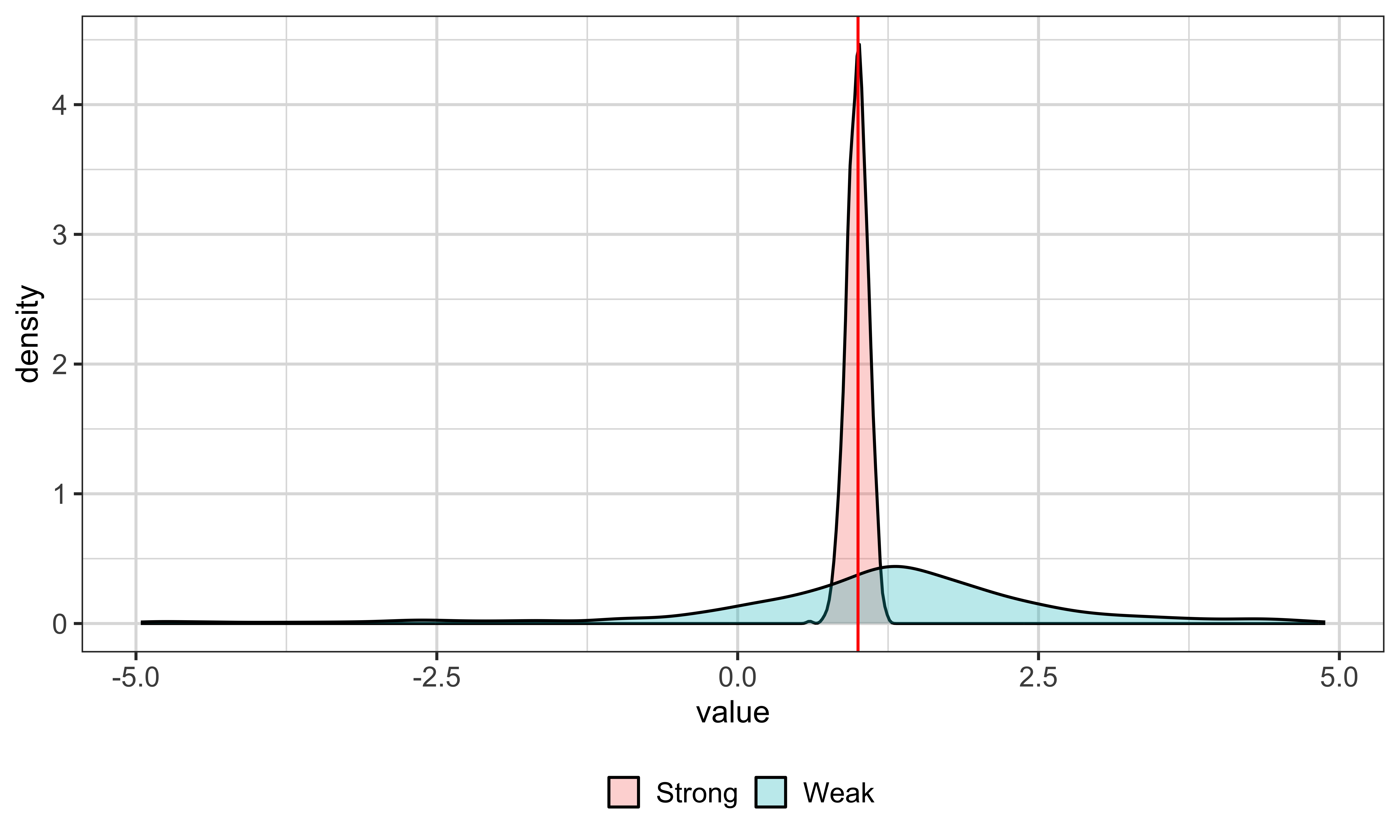
The plot omits estimates with absolute value greater than 5 so that the central portions of the distributions remain visible; extreme estimates are themselves a symptom of weak identification.
Use this final flow as a checklist for an applied IV analysis. Step one is to write the structural equation before searching for instruments. Identify the outcome, each causal coefficient of interest, all included exogenous controls, and every endogenous regressor. For each endogenous variable, explain the source of endogeneity, such as an omitted common cause, selection, reverse causality, or measurement error. That explanation tells you what the instrument must avoid.
Step two is to identify candidate excluded instruments. State the mechanism by which each candidate changes the endogenous variable and the level at which that variation occurs. Also distinguish excluded instruments from included exogenous variables, which instrument for themselves.
Step three is the blue word “argue.” Exclusion requires the instrument to affect the outcome only through the endogenous regressor, conditional on the structural controls. Exogeneity requires it to be unrelated to the structural error. Use institutional facts and a causal diagram to search for direct effects, common causes, anticipation, spillovers, or selection. Overidentification tests and placebo evidence may reveal problems, but they cannot replace this design argument.
Step four is empirical first-stage assessment. Estimate each first stage using all included exogenous variables and fixed effects from the structural specification. Show how the excluded instruments predict the endogenous regressors and report weak-identification diagnostics appropriate to the number of instruments, endogenous variables, and variance design. A first-stage relationship addresses relevance and strength, not validity.
Step five is estimation and reporting. Use a proper IV routine, choose standard errors that match clustering or other sampling dependence, and report the structural estimates together with first stages, diagnostics, identifying assumptions, and sensitivity analyses. Compare samples consistently if you contrast OLS and IV. If weak identification remains a concern, use inferential methods robust to it rather than relying only on conventional Wald output.
The order matters. A final IV coefficient is credible only when every link in this chain is credible. Software can compute the projection, but the research design supplies the causal interpretation.
Flow
Identify the endogenous variables and the exogenous controls included in the structural equation.
Identify candidate excluded instruments.
Argue why the excluded instruments satisfy exclusion and exogeneity (validity).
Assess first-stage relevance and weak-identification diagnostics (strength).
Estimate the IV model with appropriate standard errors and report the first stage, diagnostics, identifying assumptions, and sensitivity checks.