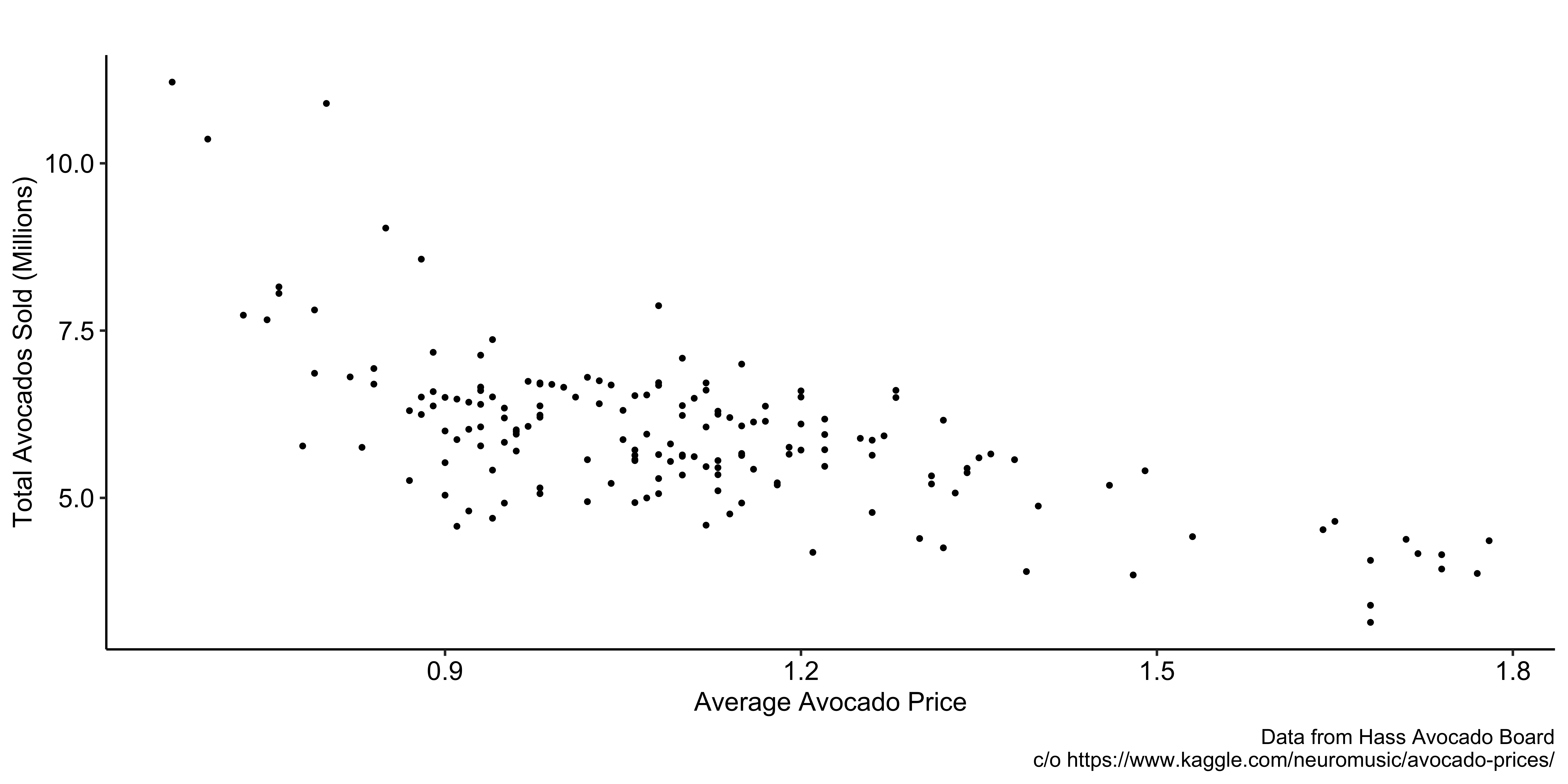
| Location | Year | P | Q |
|---|---|---|---|
| Chicago | 2003 | 75 | 2.0 |
| Peoria | 2003 | 50 | 1.0 |
| Milwaukee | 2003 | 60 | 1.5 |
| Madison | 2003 | 55 | 0.8 |
Panel data, also called longitudinal data, add a time dimension to cross-sectional data. Look at the blue word “same” in the definition. That is the defining feature. We do not merely have observations from several years. We follow the same individuals, families, firms, cities, states, or other units and observe each of them repeatedly. If we drew a new random sample of people every year, we would have repeated cross-sections, not a panel, because we could not connect one person’s later outcome to that same person’s earlier outcome.
The example gives you the basic data-collection logic. First, randomly select people from a population at one point in time. Then return to those people at later dates and reinterview them. Each person can therefore contribute several rows, with variables such as wages, hours, and education recorded in different years. A row is a person-time observation, while the person remains the cross-sectional unit.
Why is that repetition useful? It lets you compare a unit with itself. Many characteristics that differ across people or places, such as ability, geography, organizational culture, or soil type, are hard to observe but fairly stable during a study. A within-unit comparison can hold those stable characteristics fixed even when they are absent from the dataset. That possibility is the foundation for the panel estimators in this lecture.
Definition
Panel data follow the same individuals, families, firms, cities, states, or other units over time.
Example
Randomly select people from a population at a given point in time
Reinterview the same people at several later dates, producing observations on wages, hours, education, and other variables for the same group in different years.
This output makes the panel structure concrete. The first line, “data jtrain, package equals wooldridge,” loads the jtrain dataset from the wooldridge package. The next expression starts with that data, select keeps only year, factory code, employment, and sales, and the pipe passes the reduced table to head with an argument of nine. That final argument is why you see only the first nine rows rather than the entire dataset.
Read the identifiers first. fcode is the factory ID, so it tells you which rows belong to the same cross-sectional unit. year is the time index. In the displayed rows, factory 410032 appears in 1987, 1988, and 1989; then factory 410440 appears in those same three years. The unit of observation is therefore a factory-year, not merely a factory. employ is the number of employees and sales is sales in U.S. dollars. Both can change within a factory over time. For example, the first factory’s employment goes from 100 to 131 to 123, while its sales go from 47 million to 43 million to 49 million.
Whenever you receive panel data, identify the unit ID, the time ID, whether every unit appears in every period, and whether the regressors of interest actually vary within units. That last check matters because a fixed-effects coefficient is learned from within-unit change. A variable that never changes within a factory contributes no identifying variation once factory fixed effects are included.
Panel Data as data.frame
year: yearfcode: factory idemploy: the number of employeessales: sales in USDThis single question organizes the entire lecture: can the panel structure address some sources of endogeneity? The careful answer is yes, some sources, not all of them. Repeated observations let us replace comparisons across different units with comparisons of the same unit at different times. That can remove omitted characteristics that are specific to a unit and constant over time, even if we never observe those characteristics directly.
The qualification matters. Panel data do not automatically fix measurement error, simultaneous determination, reverse causality, or omitted factors that change over time. They also do not guarantee that a regressor is unrelated to future or past shocks. A fixed-effects estimate can therefore remain endogenous even after stable unit differences have been removed.
As you move through the lecture, keep asking two questions. First, what variation is actually identifying the coefficient, comparisons between units or changes within a unit? Second, which components of the error term disappear under that comparison, and which remain? The massage example in the next section makes those two questions visible with a deliberately small dataset.
Can we use the panel structure to address some sources of endogeneity?
Demand for massage (cross-sectional)
| Location | Year | P | Q |
|---|---|---|---|
| Chicago | 2003 | 75 | 2.0 |
| Peoria | 2003 | 50 | 1.0 |
| Milwaukee | 2003 | 60 | 1.5 |
| Madison | 2003 | 55 | 0.8 |
P: the price of one massageQ: the number of massages received per capitaStart by reading this as a cross-section: four locations, all observed in 2003. P is the price of one massage and Q is the number of massages received per capita. Chicago has a price of 75 and quantity of 2. Peoria has a price of 50 and quantity of 1. Milwaukee has 60 and 1.5, and Madison has 55 and 0.8. Across these four cities, the higher-price observations generally have higher quantities. The answer panel therefore correctly says that price and quantity are positively correlated.
Do not interpret that positive association as an upward-sloping demand curve. A demand effect asks what would happen to quantity if price changed while the other determinants of demand were held fixed. This table instead compares different cities, and those cities can differ in income, customer preferences, occupations, tourism, service quality, and many other ways. A regression line could accurately summarize this four-city pattern while still failing to estimate the causal response to price.
That distinction between association and causation is the identification problem. Before we can call a price coefficient a demand effect, we need variation in price that is not carrying changes in the demand environment. Flip to Question 2 and ask what omitted city characteristic could produce the positive cross-sectional pattern.
Across the four cities, how are price and quantity associated—positively or negatively?
To explain the positive correlation without claiming that higher prices cause greater demand, look for a factor with three properties. It must differ across cities, affect massages per capita, and be related to massage prices. Each item in the answer panel is a candidate.
Income can raise willingness to pay and the number of massages purchased, while also supporting higher market prices. Income is often measurable, so in principle we may be able to include it as a control. Massage quality is harder. Better-trained providers, longer sessions, or more attractive facilities can justify a higher price and also attract more customers. If quality is not measured, it remains in the error term. The physical demands of local jobs could matter too. A city with more physically taxing work may have greater demand for massage, and that stronger demand may support higher prices. Tourism, demographics, and preferences would fit the same logic.
The point is not to produce an endless list. It is to recognize that comparing Chicago with Peoria changes much more than price. The cross-city comparison does not hold the demand environment fixed, so price can be correlated with omitted determinants of quantity. On the next tab, the table reveals one of those determinants, massage quality, so you can see the confounding directly.
What could be causing the positive correlation?
The new Ql column reveals what was hidden in the first table. The code takes massage_data, pipes it into mutate, and adds a quality index with values 10, 5, 7, and 6 in the existing city order. gt then formats the resulting data frame as the table on screen. A larger value of Ql means higher massage quality.
Now compare the columns. Chicago has the highest quality index, 10, and also the highest price and quantity. Peoria has the lowest quality, 5, together with a lower price and quantity. The key says quality affects both price and massages per capita. That is exactly the structure needed for omitted-variable bias: quality belongs in the demand equation because it affects Q, and it is correlated with P because better services command different prices.
The problem callout adds the practical obstacle. Quality is not observable in this example, so we cannot simply put Ql into the real regression. Merely acknowledging that quality matters does not control for it. We would need a credible measure. The panel strategy takes another route. When we observe each city repeatedly and quality is constant within a city, we can transform the data so that the fixed quality component disappears. The next tab writes that omitted-variable problem mathematically before we introduce the repeated observations.
Demand for massage (cross-sectional)
| Location | Year | P | Q | Ql |
|---|---|---|---|---|
| Chicago | 2003 | 75 | 2.0 | 10 |
| Peoria | 2003 | 50 | 1.0 | 5 |
| Milwaukee | 2003 | 60 | 1.5 | 7 |
| Madison | 2003 | 55 | 0.8 | 6 |
Key
Massage quality was hidden (omitted) and affects both price and massages per capita.
Problem
Massage quality is not observable, and thus cannot be controlled for.
Read the first equation as follows: quantity of massages per capita, Q, equals an intercept, beta zero, plus beta one times the price of one massage, P, plus a composite error, v. Beta one is the demand effect we want. The second equation opens that composite error: v equals beta two times Ql, the unobserved quality index, plus u, which collects every other determinant of quantity not written separately.
Substituting the second line into the first would give Q equals beta zero plus beta one times P, plus beta two times quality, plus u. We estimate the shorter equation only because quality cannot be observed. That omission is not harmless. The endogeneity statement at the bottom says P is correlated with Ql. Since Ql is part of v, price is correlated with the regression error. OLS therefore cannot isolate beta one’s causal effect unless special cancellations happen.
Notice precisely what panel methods will do later. They will not recover beta two or create a measurement of quality. Instead, if quality is constant over time within each city, a within-city transformation will subtract the same beta two times quality term from itself. That removes this particular source of correlation between price and the error. It is the same omitted-variable logic from Lecture 09, now paired with a data structure that can eliminate a stable omitted factor.
Mathematically
Q=\beta_0+\beta_1P+v, \qquad v=\beta_2Ql+u
Endogeneity Problem
P is correlated with Ql.
| Location | Year | P | Q | Ql |
|---|---|---|---|---|
| Chicago | 2003 | 75 | 2.0 | 10 |
| Chicago | 2004 | 85 | 1.8 | 10 |
| Peoria | 2003 | 50 | 1.0 | 5 |
| Peoria | 2004 | 48 | 1.1 | 5 |
| Milwaukee | 2003 | 60 | 1.5 | 7 |
| Milwaukee | 2004 | 65 | 1.4 | 7 |
| Madison | 2003 | 55 | 0.8 | 6 |
| Madison | 2004 | 60 | 0.7 | 6 |
The table above now has two observations for each of four cities, one in 2003 and one in 2004. The data-building code makes that structure deliberately. rep with each equal to two repeats each location twice, while the year vector alternates 2003 and 2004 for each city. The price and quantity vectors supply a value for every city-year. Quality is also repeated twice within each city, so Chicago remains at 10 in both years, Peoria at 5, Milwaukee at 7, and Madison at 6.
That panel contains the two kinds of variation listed on screen. Intercity, or between-city, variation compares different cities, such as Chicago with Peoria. Intracity, or within-city, variation compares one city with itself over time, such as Chicago in 2004 with Chicago in 2003. A single cross-section offers only the first kind because each city appears once. A pooled regression on the two-year table can mix both kinds.
Our objective is to discard the between-city component that carries the persistent quality differences and use only the within-city changes. Quality varies across cities, but within a city its change is exactly zero by construction. That is why the panel structure can help here. Move to the within-city tab and read the price and quantity changes row by row.
There are two kinds of variation:
Cross-sectional data offer only between-city variation.
Compare the two years within each city rather than comparing one city with another. In Chicago, price rises from 75 to 85 while massages per capita fall from 2 to 1.8. In Peoria, price falls from 50 to 48 while quantity rises from 1 to 1.1. In Milwaukee, price rises from 60 to 65 and quantity falls from 1.5 to 1.4. In Madison, price rises from 55 to 60 and quantity falls from 0.8 to 0.7. Every within-city movement therefore points to a negative association: higher price accompanies lower quantity, and the one price decrease accompanies a quantity increase.
That negative within-city association coexists with the positive cross-city association from the earlier tab. There is no paradox because the comparisons hold different things fixed. The between comparison asks why cities with different price levels also have different quantity levels. The within comparison asks what happens when price changes relative to the same city’s earlier price. Since the constructed quality index stays constant within a city, quality cannot explain those year-to-year movements.
This is why the source of variation matters as much as the sign of a coefficient. A positive pooled association can be driven by stable quality differences, while the within relationship can be negative. The question on the next tab asks you to state exactly why the within comparison is more credible here, and also to state its limit.
Now, compare the massage price and massages per capita within each city (over time). What do you see?
Looking within a city helps because it holds fixed every city characteristic that is exactly constant over the two observed years. In this constructed example, massage quality is one of those characteristics. Chicago’s quality is 10 in both periods, so when we compare Chicago in 2004 with Chicago in 2003, the quality difference is zero. The same is true for every other city. Quality therefore cannot be the reason that a city’s price and quantity changed between these two dates.
That is the precise answer behind the answer panel: restricting attention to within-city variation removes confounding from this time-invariant omitted variable. It also removes other stable city features, even features we did not name, because each is compared with itself.
Do not broaden the conclusion beyond what the comparison earns. If income changes within a city, if massage quality itself changes, or if a temporary festival raises demand and price in the same year, those time-varying factors can remain in the error and remain correlated with price. Reverse causality can remain as well. Panel data create an opportunity to make cleaner comparisons, but they do not make every price change exogenous. The next section shows how to force a regression to use only this within-city variation, first by taking first differences.
Why does looking at within-city variation seem to help us estimate the effect of massage price on demand more credibly?
First differencing is the first regression method for isolating the within-city movement. Instead of using the levels of price and quantity, compute delta P and delta Q, meaning the later value minus the earlier value for the same city, and regress the change in quantity on the change in price.
Follow the code that builds the displayed table. It starts with the two-period massage data, then group_by Location tells every subsequent lag and subtraction to operate separately within each city. Inside mutate, P_dif is price minus lagged price, Q_dif is quantity minus lagged quantity, and Ql_dif is quality minus lagged quality. lag means the preceding row within that city’s group. ungroup removes the grouping after those new columns have been created, preventing it from accidentally affecting later operations.
The first observation for each city has no preceding observation, so each difference is missing there. The orange cells in the second row of each city contain the usable changes. For Chicago, delta price is 10 and delta quantity is negative 0.2. For Peoria they are negative 2 and positive 0.1. Quality’s difference is zero for every city because its two values are identical.
Regressing delta Q on delta P therefore discards every difference in fixed city levels. The key in the right column emphasizes why this works for our confounder: constant quality subtracts to zero. The next tab derives the same cancellation equation by equation.
Question
How do we use only within-city variation in a regression framework?
First differencing
One approach is to compute the changes in price and quantity within each city (\Delta P and \Delta Q) and then regress \Delta Q on \Delta P.
First-differenced Data
| Location | Year | P | Q | Ql | P_dif | Q_dif | Ql_dif |
|---|---|---|---|---|---|---|---|
| Chicago | 2003 | 75 | 2.0 | 10 | NA | NA | NA |
| Chicago | 2004 | 85 | 1.8 | 10 | 10 | -0.2 | 0 |
| Peoria | 2003 | 50 | 1.0 | 5 | NA | NA | NA |
| Peoria | 2004 | 48 | 1.1 | 5 | -2 | 0.1 | 0 |
| Milwaukee | 2003 | 60 | 1.5 | 7 | NA | NA | NA |
| Milwaukee | 2004 | 65 | 1.4 | 7 | 5 | -0.1 | 0 |
| Madison | 2003 | 55 | 0.8 | 6 | NA | NA | NA |
| Madison | 2004 | 60 | 0.7 | 6 | 5 | -0.1 | 0 |
Key
Variation in quality is eliminated after first differencing because quality is constant within each city.
The subscripts in the first line separate the two dimensions of a panel. i identifies the city and t identifies time. Quantity for city i at time t equals beta zero, plus beta one times that city’s price at that time, plus beta two times its quality at that time, plus u i t, all other determinants of quantity for that city and date.
The next two lines write that model once for period one and once for period two. To first-difference, subtract the entire period-one equation from the entire period-two equation. On the left, Q i 2 minus Q i 1 is delta Q i. The two beta-zero intercepts cancel. The price terms become beta one times P i 2 minus P i 1, which is beta one times delta P i. Quality becomes beta two times delta Ql i, and the remaining errors become delta u i, meaning u i 2 minus u i 1. That justifies every term in the third displayed line.
Now use the special assumption in blue below it. Quality is the same in periods one and two, so delta quality equals zero. Beta two times zero disappears, leaving delta quantity equals beta one times delta price plus delta u. This removes endogeneity caused by time-invariant massage quality.
It does not establish causality by itself. We still need delta price to be uncorrelated with delta u. A temporary demand shock, a change in quality, or reverse causality could make the two changes move together. First differencing solves a specific stable-omitted-variable problem, not every source of endogeneity.
A new way of writing a model
Q_{i,t}=\beta_0+\beta_1P_{i,t}+\beta_2Ql_{i,t}+u_{i,t}
i: indicates cityt: indicates timeFirst differencing
Q_{i,1}=\beta_0+\beta_1P_{i,1}+\beta_2Ql_{i,1}+u_{i,1}
Q_{i,2}=\beta_0+\beta_1P_{i,2}+\beta_2Ql_{i,2}+u_{i,2}
\Rightarrow
\Delta Q_i=\beta_1\Delta P_i+\beta_2\Delta Ql_i+\Delta u_i
Endogeneity Problem?
Since Ql_{i,1}=Ql_{i,2}, \Delta Ql_i=0, so
\Delta Q_i=\beta_1\Delta P_i+\Delta u_i.
First differencing removes endogeneity caused by time-invariant massage quality. It does not remove endogeneity from time-varying omitted factors or reverse causality; we still need \Delta P_i to be uncorrelated with \Delta u_i.
The small data display first lets you verify the difference columns. head with five shows the first five rows, including both observations for Chicago and Peoria and the first Milwaukee observation. Difference values are missing in each city’s first row because there is no prior year.
The left regression calls feols with Q on P using the data frame massage_data_fd. Even though this object contains difference columns, the formula uses the original level variables. tidy converts the fitted model into a term-by-term table. Using all eight city-year observations, the price coefficient is about positive 0.0287. That regression mixes between-city level differences with within-city changes, so the stable quality differences can drive a positive estimate.
The right regression changes the formula to Q_dif on P_dif. feols drops the four first-year rows whose differences are missing, leaving one change for each city. The estimated price-change coefficient is about negative 0.0253. The formula includes an intercept, estimated at about 0.039, so this specification allows a common change in quantity when the price change is zero. That detail matters later: a two-period demeaned regression without a time effect need not match this intercept-included first-difference slope.
With only four usable changes, neither standard errors nor significance should be treated as empirical evidence. The demonstration is about identification. Differencing removes fixed cross-city quality levels, changes the comparison behind the coefficient, and reverses the sign in this constructed example.
Data
OLS on the original data:
OLS on the first-differenced data:
The three bullets summarize the logic of the entire two-period example. First, suppose an omitted variable affects both the dependent variable and the independent variable, creating endogeneity in a cross-sectional regression. If that omitted variable is constant over time within each unit, comparing a unit with itself subtracts the omitted level from itself. In the massage example, quality affects both quantity and price, but its within-city change is zero.
Second, first differencing operationalizes that comparison. Replace every level with period two minus period one, then regress changes in the outcome on changes in the explanatory variable. All between-unit level variation disappears. A city whose price never changes supplies no identifying variation for beta one, even though its row may still help with other parts of a larger model.
Third, this is possible only because the same cross-sectional units are observed at multiple times. With a different sample of cities each year, we could not form a city-specific change. That is the distinctive value of panel data.
Keep the limitation attached to the conclusion. Differencing removes fixed omitted factors, but it does not remove omitted factors that change over time, measurement error, or reverse causality. The change in the regressor still needs to be unrelated to the change in the remaining error. With more than two periods, we could form successive differences, but the next section introduces a convenient alternative: deviations from each unit’s time average.
When an omitted variable affecting both the dependent and independent variables is constant over time, using within-unit variation can eliminate the bias caused by that variable.
First-differencing the data and regressing changes on changes removes between-unit variation.
Of course, first-differencing is possible only because the same cross-sectional units are observed multiple times over time.
With many years, we could calculate 2004 minus 2003, 2005 minus 2004, and every other successive first difference, then combine those changes in one regression. The slide proposes a more convenient representation. For every city and every variable, calculate the city’s time average and subtract that average from each city-year observation. This is the within transformation, also called demeaning.
Follow the data construction. The first select keeps Location, Year, price, quantity, and quality. group_by Location makes every mean city-specific rather than an average over all cities. Inside mutate, P_mean is a city’s mean price and P_dev is observed price minus that mean. The same two steps create the quantity mean and deviation, and the quality mean and deviation. ungroup ends the city grouping. The final select does not change values; it arranges each original variable next to its mean and deviation for the displayed table. The orange styling highlights the three deviation columns.
Interpret those columns relative to each city’s usual level. A positive price deviation means that city’s price is above its own time average, not above the average price across cities. A negative quantity deviation means quantity is below that city’s usual quantity. For Chicago, whose prices are 75 and 85, the mean is 80 and the deviations are negative 5 and positive 5. Because quality is constant within every city, each quality value equals its own city mean, so every Ql_dev is zero. Those deviations are the inputs to the fixed-effects regression on the next tab.
Within transformation
If we have lots of years of data, we could, in principle, compute all of the first differences (i.e., 2004 versus 2003, 2005 versus 2004, etc.) and then run a single regression. But there is an easier way.
Instead of thinking of each year’s observation in terms of how much it differs from the prior year for the same city, let’s think about how much each observation differs from the average for that city.
Example
How much does each observation differ from its city average?
| Location | Year | P | P_mean | P_dev | Q | Q_mean | Q_dev | Ql | Ql_mean | Ql_dev |
|---|---|---|---|---|---|---|---|---|---|---|
| Chicago | 2003 | 75 | 80.0 | -5.0 | 2.0 | 1.90 | 0.10 | 10 | 10 | 0 |
| Chicago | 2004 | 85 | 80.0 | 5.0 | 1.8 | 1.90 | -0.10 | 10 | 10 | 0 |
| Peoria | 2003 | 50 | 49.0 | 1.0 | 1.0 | 1.05 | -0.05 | 5 | 5 | 0 |
| Peoria | 2004 | 48 | 49.0 | -1.0 | 1.1 | 1.05 | 0.05 | 5 | 5 | 0 |
| Milwaukee | 2003 | 60 | 62.5 | -2.5 | 1.5 | 1.45 | 0.05 | 7 | 7 | 0 |
| Milwaukee | 2004 | 65 | 62.5 | 2.5 | 1.4 | 1.45 | -0.05 | 7 | 7 | 0 |
| Madison | 2003 | 55 | 57.5 | -2.5 | 0.8 | 0.75 | 0.05 | 6 | 6 | 0 |
| Madison | 2004 | 60 | 57.5 | 2.5 | 0.7 | 0.75 | -0.05 | 6 | 6 | 0 |
Note
We call this transformation the within transformation, or demeaning.
This tab states the fixed-effects model in terms of the columns we just created. The dependent variable is Q_dev, quantity in a city-year minus that city’s mean quantity. The independent variable is P_dev, price in that city-year minus that city’s mean price. The regression therefore asks: when a city’s price is above or below its own usual price, is its quantity also above or below its own usual quantity?
The key explains why quality is absent. Ql is constant within each city, so the city-specific quality mean equals every observed quality value. Ql_dev, defined as quality minus its city mean, is zero in every row. A column of zeros cannot explain variation or generate omitted-variable bias in the transformed equation. Stable income, geography, or preferences would disappear in the same way, whether or not we observed and named them.
This is the multi-period version of comparing a city with itself. It discards information about whether Chicago has a higher average price or quantity than Peoria and keeps only deviations around each city’s own average. The following tab derives this transformation from the original equations, so look for the intercept and the city-specific quality component canceling when the average equation is subtracted.
Model
Q_devP_devKey
Because Ql is constant within each city, demeaning makes Ql_dev equal to zero.
The first group of equations writes one demand equation for city i in every period from one through capital T. In each line, quantity equals beta zero, plus beta one times price, plus beta two times quality, plus the remaining error. The vertical dots mean the same equation exists for every intermediate period.
Now average all capital T equations for a particular city. Its average quantity is bar Q i, its average price is bar P i, its average quality is bar Ql i, and its average error is bar u i. Beta zero remains beta zero because averaging the same intercept capital T times leaves it unchanged. Next, subtract that city-average equation from the equation for a particular time t.
On the left you get Q i t minus bar Q i. The two intercepts cancel. The price contribution becomes beta one times the quantity P i t minus bar P i. Quality becomes beta two times Ql i t minus bar Ql i. The error becomes u i t minus bar u i. That is exactly the last displayed equation.
Notice that the disturbance is demeaned too. Bar u i includes errors from every period for city i, so the transformed regressor’s relationship to shocks in other periods will matter for unbiasedness. We keep the quality-deviation term visible on this tab to show the algebra; flip to the next tab to apply the assumption that quality never changes.
Q_{i,1}=\beta_0+\beta_1P_{i,1}+\beta_2Ql_{i,1}+u_{i,1}
Q_{i,2}=\beta_0+\beta_1P_{i,2}+\beta_2Ql_{i,2}+u_{i,2}
\vdots
Q_{i,T}=\beta_0+\beta_1P_{i,T}+\beta_2Ql_{i,T}+u_{i,T}
\Rightarrow
Q_{i,t}-\bar Q_i=\beta_1(P_{i,t}-\bar P_i)+\beta_2(Ql_{i,t}-\overline{Ql}_i)+(u_{i,t}-\bar u_i)
The first line states the time-invariance assumption explicitly. For a given city i, quality in period one equals quality in period two, and so on through period capital T; all of them equal that city’s average quality. Therefore Ql i t minus bar Ql i is zero in every period.
Apply that result to the transformed equation from the previous tab. Beta two times the quality deviation is beta two times zero, so it disappears. The remaining equation says quantity minus its city mean equals beta one times price minus its city mean, plus the error minus its city mean. Price may still be correlated with the level of quality across cities, but the regression no longer uses those between-city level differences. That particular endogeneity channel has been removed.
The question mark in the heading is important because other endogeneity can survive. A temporary demand shock could raise both quantity and the market price in one period. A city-specific promotion could change quality and price together. Either case could leave demeaned price correlated with the demeaned error. The within transformation removes time-invariant Ql; it does not prove that all remaining price variation is exogenous. We now generalize the same algebra by collecting every stable unit characteristic into one fixed effect, alpha i.
Ql_{i,1}=Ql_{i,2}=\dots=Ql_{i,T}=\overline{Ql}_i
\Rightarrow
Q_{i,t}-\bar Q_i=\beta_1(P_{i,t}-\bar P_i)+(u_{i,t}-\bar u_i)
The within transformation removes the endogeneity caused by time-invariant Ql. Other sources of endogeneity may remain.
Consider the following general model
y_{i,t}=\beta_1 x_{i,t} + \alpha_i + u_{i,t}
Start with the general panel model shown above the tabs. y i t is the outcome for unit i at time t. x i t is the explanatory variable, and beta one is its slope. Alpha i is the individual fixed effect: one combined term representing all unobserved, time-invariant factors specific to unit i. The last term, u i t, contains factors that can vary across both units and time. There is no separate intercept in this notation because any common intercept can be included in alpha i.
Crucially, the slide allows alpha i to be correlated with x i t. Pooled OLS would put alpha i in the error and require that correlation to be zero. Fixed effects is designed precisely to avoid that requirement.
Look at the averaging step. For a given unit, add its capital T equations and divide by capital T. One over T times the sum of y i t becomes bar y i, the time average for unit i; the corresponding averages are bar x i and bar u i. Beta one is constant, so it factors outside the average. Alpha i is repeated unchanged in every period, and its average is still alpha i, as the note on the last line shows. The bars are averages over time within one individual, not averages across different individuals. The next tab subtracts this average equation from each original observation.
For each i, averaging this equation over time gives
\frac{1}{T}\sum_{t=1}^T y_{i,t}=\beta_1\frac{1}{T}\sum_{t=1}^T x_{i,t}+\alpha_i+\frac{1}{T}\sum_{t=1}^T u_{i,t}
We use \bar z_i to denote the time average of z_{i,t} for unit i. Thus,
\bar y_i=\beta_1\bar x_i+\alpha_i+\bar u_i.
Note that \frac{\sum_{t=1}^T \alpha_{i}}{T} = \alpha_i
Take the original observation-level equation and subtract the unit-average equation term by term. On the left, the result is y i t minus bar y i. For the regressor it is beta one times x i t minus bar x i. The time-varying disturbance becomes u i t minus bar u i. Finally, the fixed effect appears as alpha i minus alpha i.
The important callout emphasizes the decisive cancellation: alpha i is gone. Every stable unit characteristic collected in alpha i subtracts from itself, including characteristics we cannot observe or even name. We do not need to estimate a coefficient for ability, geography, culture, soil type, or each other component separately.
The same cancellation also creates an identification cost. Any observed regressor that is constant within a unit has a within deviation of zero, just like alpha i. Its coefficient cannot be separately estimated in a model with unit fixed effects. Fixed effects also cannot remove an omitted factor that changes over time, because that factor belongs in u i t rather than alpha i. What remains is an ordinary-looking regression in demeaned variables, which is the estimation step on the next tab.
Subtracting the equation of the average from the original model,
y_{i,t}-\bar y_i=\beta_1(x_{i,t}-\bar x_i)+(u_{i,t}-\bar u_i)+\alpha_i-\alpha_i
Important
\alpha_i is gone!
After the within transformation, regress y i t minus bar y i on x i t minus bar x i using OLS. The coefficient on the demeaned regressor estimates beta one. There is no alpha i term left to include because the transformation eliminated it.
Interpret beta one as a within-unit relationship. When x is one unit above its usual value for the same individual, how far is y from that individual’s usual outcome, holding the other included regressors fixed? The estimate does not compare a person with high average x to a different person with low average x. All purely between-person variation has been removed.
This also tells you where the information comes from. If a unit’s x is constant across all dates, every value of x i t minus bar x i is zero, so that unit supplies no identifying variation for beta one. Units with larger useful within changes generally contribute more information. In real applications, software performs the demeaning or an equivalent absorption algorithm internally, so you normally keep variables in their original units rather than manually creating every deviation. Before using the coefficient causally, however, we still need an exogeneity condition for the transformed error. That is the question on the next slide.
We then regress (y_{i,t}-\bar{y}_i) on (x_{i,t}-\bar{x}_i) to estimate \beta_1.
The transformed model at the top says demeaned y equals beta one times demeaned x plus demeaned u. Removing alpha i is necessary, but it is not enough for an unbiased fixed-effects estimate. We need x i t minus bar x i to be uncorrelated with u i t minus bar u i.
Why is a condition involving only the current period not sufficient? Both bars are constructed from every period. Bar x i contains past and future regressor values, and bar u i contains past and future shocks. Correlation between a current shock and a future x can therefore enter the transformed variables.
The callout gives a standard sufficient condition called strict exogeneity. Say it as: the expected value of u i t, conditional on the entire sequence x i 1, x i 2, through x i T, and conditional on alpha i, equals zero for every time t. Capital E is conditional expectation, and the vertical bar means “given.” This requires regressors in every period to be unrelated to the shock in every period. The example E of u i 1 given x i 4 and alpha i equals zero shows that even a period-one shock must not predict the period-four regressor.
Strict exogeneity rules out contemporaneous omitted shocks and feedback from today’s outcome shock into future choices of x. If an unexpected increase in y this year causes the unit to change x next year, the condition fails. Fixed effects removed stable heterogeneity, but it did not solve that dynamic feedback problem.
Here is the model after within-transformation:
\begin{align*} y_{i,t}-\bar{y}_i=\beta_1 (x_{i,t} -\bar{x}_i) + (u_{i,t} -\bar{u}_i) \end{align*}So,
x_{i,t}-\bar x_i must be uncorrelated with u_{i,t}-\bar u_i.
Strict exogeneity
A sufficient condition is
E[u_{i,t}\mid x_{i,1},x_{i,2},\dots,x_{i,T},\alpha_i]=0 \qquad\text{for every }t.
Thus, regressors in any period must be unrelated to shocks in every period. For example, E[u_{i,1}\mid x_{i,4},\alpha_i]=0.
This command applies ordinary least squares to the within-transformed massage variables we created earlier. It calls the feols function from the fixest package. Read the formula aloud as “Q underscore dev on P underscore dev”: the quantity-deviation column is the dependent variable and the price-deviation column is the explanatory variable. The data argument points to the within-transformed massage table. Because these columns are already deviations from city means, we do not name a fixed-effect identifier after a vertical bar in this particular call.
The fitted price-deviation coefficient is about negative 0.0208. Interpret it within cities: when price is one dollar above a city’s own two-year average, predicted massages per capita are about 0.0208 below that city’s own average, in this constructed dataset. The intercept is essentially zero because demeaned variables have zero means.
With two periods, first differences and within deviations encode the same pairwise movements, but specifications must treat common time changes consistently to produce identical slopes. The earlier first-difference code included an intercept, while this demeaned regression has no year effect corresponding to that common change, so its displayed slope is not the earlier negative 0.0253. That is a specification detail, not a contradiction in the idea of within variation. In practice, we normally let fixed-effects software work from the original variables rather than constructing deviations by hand.
Fixed effects estimation
Regress within-transformed Q on within-transformed P:
The slide compares two mathematically equivalent ways to account for unit-specific intercepts. The first is the within estimator we just derived: subtract each unit’s time average from every observation, then run OLS on the demeaned outcome and regressors. The second is the least-squares dummy-variable approach: keep the variables in their original levels and include indicator variables for the units.
Why are they equivalent? A complete set of unit indicators allows every unit to have its own intercept. OLS then removes each unit’s fitted level before choosing the common slope, which is the same within-unit variation produced by demeaning. When the outcome, regressors, sample, and other effects are specified consistently, both approaches produce exactly the same slope estimates.
Each view is useful. Demeaning makes the identifying variation transparent because you can literally see deviations from unit means. Dummy variables make the different unit intercepts explicit. In a small four-city example we can create the indicators ourselves, but with thousands or millions of units that would be wasteful and error-prone. Modern fixed-effects software absorbs the indicators algebraically without building a huge visible dummy matrix. The next two tabs demonstrate the dummy-variable version and the omitted reference category.
Important
The two approaches below will result in the same coefficient estimates (mathematically identical).
You can use the original data (no within-transformation) and include dummy variables for all the cities except one.
The code starts with the original two-period massage data and pipes it to mutate, which adds three indicator variables. For each row, ifelse tests whether Location equals the named city. It returns one when the condition is true and zero otherwise. Peoria_D therefore marks Peoria rows, Milwaukee_D marks Milwaukee rows, and Madison_D marks Madison rows. The parentheses around the assignment cause R to save the result as massage_data_d and print it, so you can inspect the new zero-one columns.
There are four cities, but the code creates only three indicators because the regression will also contain an intercept. Chicago is the omitted reference category: when all three displayed indicators equal zero, the row belongs to Chicago. Each included dummy permits its city’s intercept to differ from Chicago’s intercept.
If we included indicators for all four cities together with an intercept, the four dummies would sum to one in every row, exactly duplicating the intercept column. That perfect multicollinearity is the dummy-variable trap. Omitting one category solves it without losing any fitted values. These city indicators absorb every characteristic that is constant within a city, not only the quality index we happened to name. Flip to the next tab to put them into the level regression and compare the price slope with the demeaned result.
This feols call uses the original quantity Q as the dependent variable and the original price P as the main regressor. The plus signs add the Peoria, Milwaukee, and Madison indicators. data equals massage_data_d supplies the table we created on the previous tab. Because Chicago has no included indicator, the ordinary intercept is Chicago’s city-specific intercept, and each dummy coefficient is that city’s intercept difference relative to Chicago, holding price fixed.
Focus on the price estimate. It is about negative 0.0208, exactly the coefficient from regressing Q_dev on P_dev. The equality is the empirical demonstration of the algebraic equivalence stated on the previous slide. The dummy coefficients, about negative 1.49 for Peoria, negative 0.81 for Milwaukee, and negative 1.62 for Madison, capture stable level differences relative to Chicago in this constructed equation. They are nuisance parameters here, not the causal target.
Their purpose is to stop persistent cross-city differences from influencing the common price slope. Once each city has its own intercept, the slope is chosen from price and quantity movement within cities. With many units, you would not manually write all these dummy names. The next section shows the fixed-effect syntax that absorbs them directly.
Note that the coefficient estimate on P is exactly the same as the one we saw earlier when we regressed Q_dev on P_dev.
The sentence at the top gives the substantive meaning of the algebra. When you include individual dummies, or individual fixed effects, you remove differences between the units’ average levels. In the massage example, city fixed effects prevent the regression from using the fact that Chicago has a higher average price and quantity than Peoria. Beta one is identified from price and quantity movement within the same city over time.
The callout generalizes the rule. Fixed effects for a category absorb differences between the groups in that category and identify the remaining coefficients from variation within those groups. Firm fixed effects use within-firm changes and absorb stable differences between firms. Farmer fixed effects use within-farmer changes and absorb stable differences between farmers. Month-year fixed effects, which appear later in the avocado example, compare weeks within the same calendar month.
This is not a mechanical instruction to include whichever fixed effect is available. The right grouping follows from the data-generating process. Ask where the troublesome unobserved factors operate and which comparisons the research design claims are clean. Fixed effects can improve credibility when stable between-group differences confound the raw relationship, but they cannot rescue variation that is endogenous within the chosen groups.
By including individual dummies (individual fixed effects), you effectively remove between-city variation and estimate \beta_1 using within-city variation.
Very important
More generally, including fixed effects for a category (such as city) absorbs differences between its groups and identifies other coefficients from variation within those groups.
The advice on screen is practical: do not manually demean every variable, and do not manually create a dummy for every unit. Both are useful for understanding the estimator, but both invite coding mistakes and become cumbersome in real panels. Use the fixest package and let feols absorb the fixed effects efficiently.
Read the syntax from left to right. The first part explicitly calls feols from the fixest package. Say the formula as “dependent variable tilde independent variables, vertical bar fixed effect.” The dependent-variable placeholder before the tilde is the untransformed outcome. The independent-variables placeholder after the tilde is the list of untransformed regressors whose coefficients you want. The vertical bar separates ordinary slope regressors from fixed-effect identifiers. The fixed-effect placeholder is the variable identifying the repeatedly observed cross-sectional unit, such as Location in the massage panel. The final data argument supplies the data frame containing all those columns.
Internally, the software obtains the same slope as the correctly specified within or dummy-variable estimator, without forcing you to store transformed columns or thousands of indicators. The output can also report how many fixed-effect groups and observations were used. Syntax does not choose a research design for you, however. You must still justify why the fixed-effect grouping absorbs the relevant confounders and why the remaining within-group variation is exogenous. The next tab applies this syntax to the massage data.
Advice
In practice
We will use the fixest package.
Syntax
FE: the name of the variable that identifies the cross-sectional units that are observed over time (Location in our example)dep_var: untransformed dependent variableindep_vars: list of (non-transformed) independent variablesThe first output displays massage_data_2p in its original form. There are eight rows, two years for each of four locations, with the original price, quantity, and quality columns. Nothing has been manually demeaned and no city dummies have been added.
The second cell sends those original variables directly to feols. The formula says Q on P, then the vertical bar introduces Location as the fixed-effect identifier. data equals massage_data_2p supplies the eight observations. The estimator absorbs four location effects and reports a price coefficient of about negative 0.0208. That exactly matches both the earlier Q_dev on P_dev regression and the level regression with three explicit city dummies.
Use that equality as a syntax check while learning: manual demeaning, a complete nonredundant set of unit indicators, and absorption should agree when the specifications and samples are the same. The output also reports eight observations, four Location fixed-effect groups, and a within R-squared of about 0.95. In an actual application, inspect those sample and group counts and verify that each regressor has useful within-group variation. A command can run successfully even when the identifying changes are too sparse or too narrowly concentrated to support a credible claim.
Data
Example
Random effects, abbreviated R E, offers a different treatment of alpha i. Fixed effects allows alpha i to be correlated with the explanatory variables and removes it through within-unit comparisons. Random effects instead assumes that alpha i is uncorrelated with every explanatory variable in every period. That is a stronger orthogonality assumption, and it must come from the research design, not from the estimator’s name.
Under that assumption, random effects consistently combines within-unit and between-unit information. Because it retains between variation, it can be more efficient than fixed effects, meaning it may produce smaller sampling variance. It can also estimate coefficients on time-invariant regressors, whose within deviations would be zero under unit fixed effects.
The cost is vulnerability to a failed assumption. If stable unobserved ability, geography, management quality, or another component of alpha i is correlated with the regressors, standard random effects is inconsistent. Fixed effects can still be consistent if the strict-exogeneity condition for the time-varying error holds. You should therefore choose between F E and R E based on knowledge of how x is assigned and whether correlation with stable unit traits is plausible. Do not choose R E simply because it reports smaller standard errors, and do not treat a specification test as a substitute for substantive reasoning. This lecture stops at that comparison and does not develop R E estimation further.
How is it different from the FE model?
Random effects (RE) assumes \alpha_i is uncorrelated with every explanatory variable in every period.
Under that assumption, RE is consistent and can be more efficient than FE. It can also estimate coefficients on time-invariant regressors.
If \alpha_i is correlated with the explanatory variables, the standard RE estimator is inconsistent, whereas FE remains consistent under strict exogeneity.
The choice between FE and RE should be based on the research design and the plausibility of the RE orthogonality assumption.
Note
We do not develop RE estimation further in this lecture.
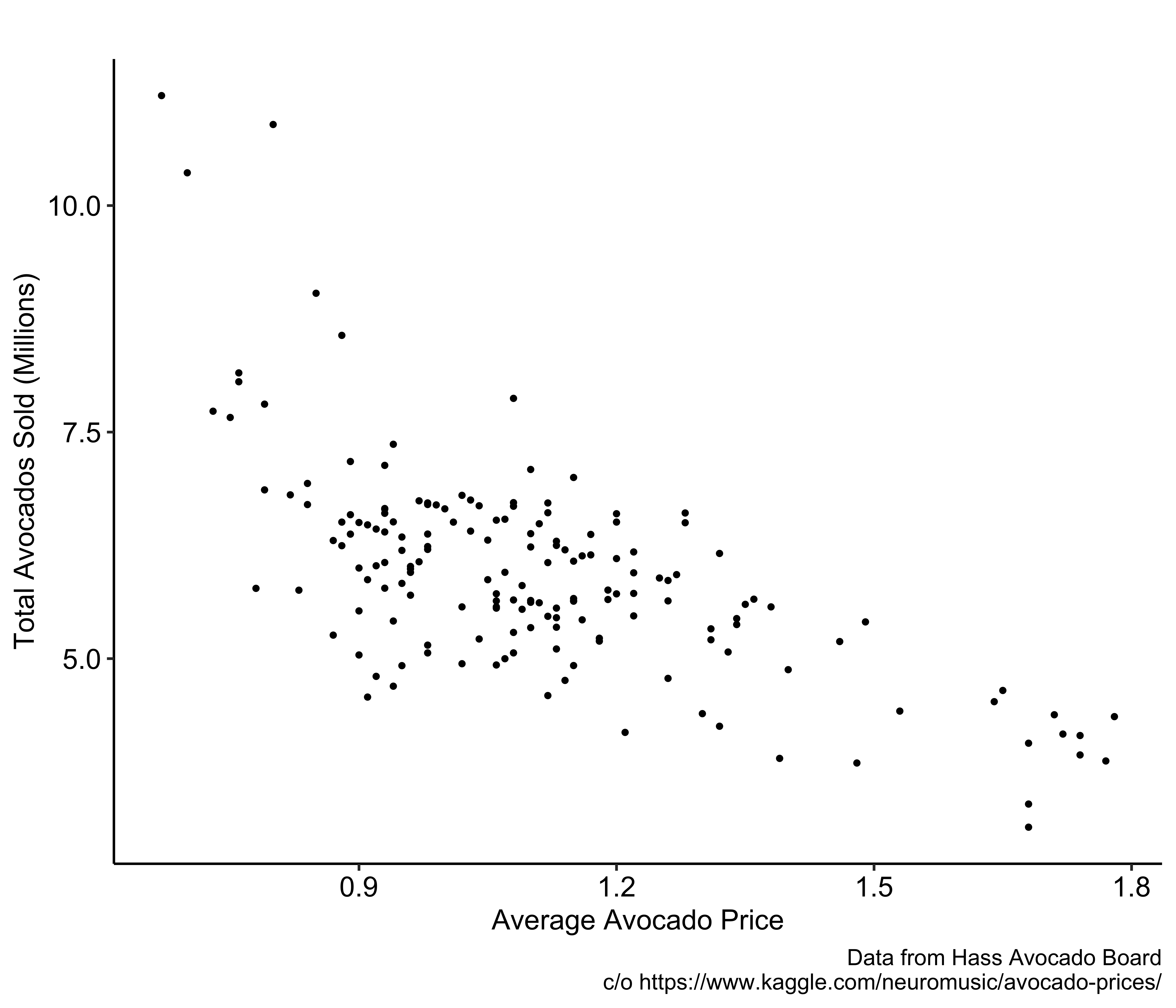
This application asks how avocado consumption responds to price, using weekly observations for conventional avocados in California from January 2015 through March 2018. The data code reads avocado.csv with fread, filters to rows whose region is California and whose type is conventional, divides Total Volume by one million to create a more readable sales measure, and orders the rows by Date. Those choices define the sample and units shown in the figure.
Now read the plot. The horizontal axis is Average Avocado Price. The vertical axis is Total Avocados Sold in millions. Each point is one week, drawn with a small point size of 0.8 because there are 169 weekly observations. The lecture theme controls the appearance, while labs supplies the axis labels, removes a title with an empty string, and credits the Hass Avocado Board data source in the caption. The point cloud slopes downward overall: weeks with higher average prices tend to have lower sales volumes.
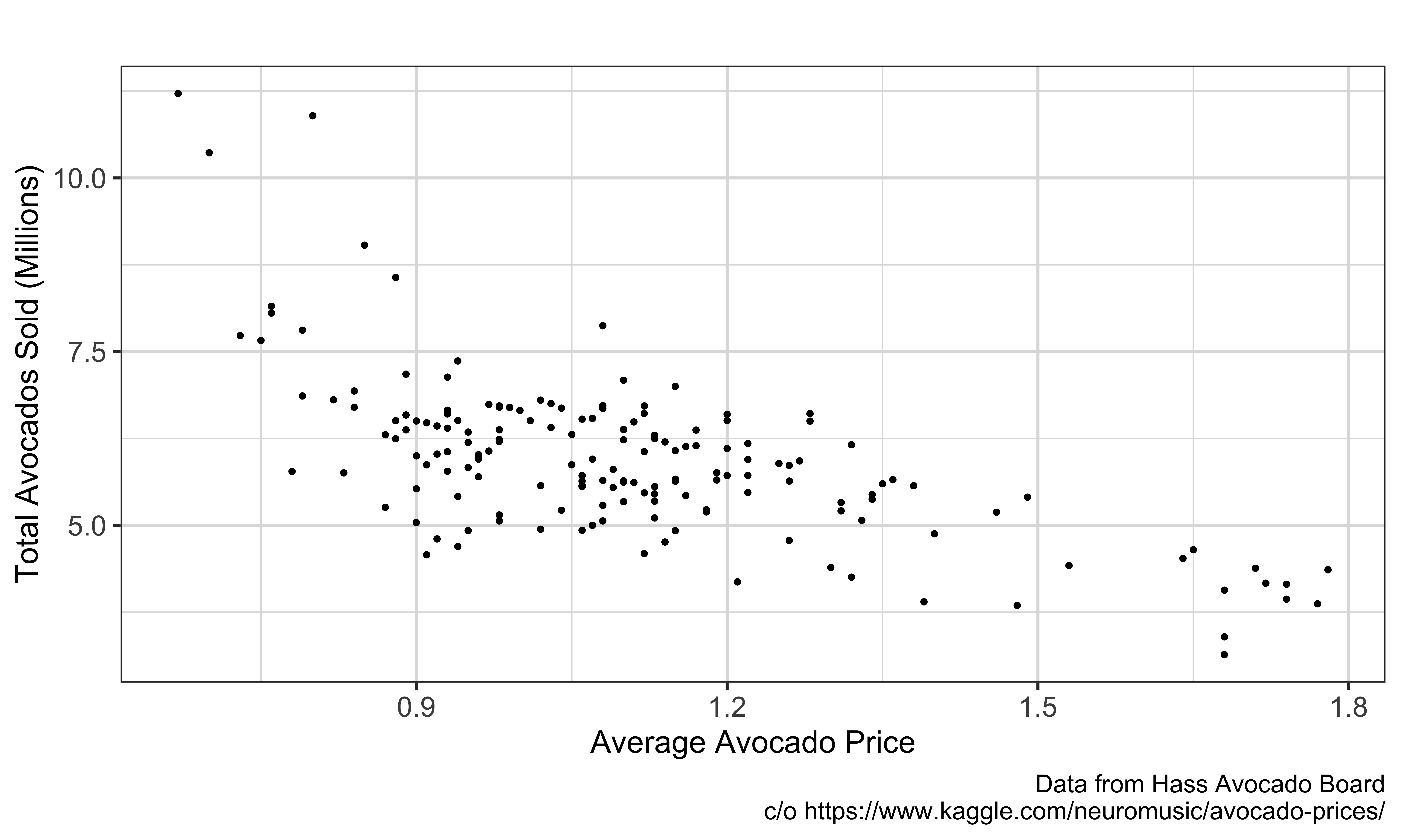
That picture is descriptive, not yet a causal demand curve. Market price is an equilibrium outcome jointly determined by supply and demand. Weather or a supply disruption can change available quantity and price together. Promotions, holidays, or changing preferences can shift demand and affect both observed price and sales. Our objective is the effect of a price change on consumption, so we need price variation that is plausibly unrelated to unobserved demand shocks. The next tab makes the simultaneity problem explicit.

Objective
You are interested in understanding the impact of avocado price on its consumption.
The observations in the left column describe the same negative pattern you see in the scatterplot on the right. Sales tend to be lower in high-price weeks, and, reading the relationship in the other direction, prices tend to be higher in weeks when fewer avocados are sold. The second plotting cell redraws g_avocado; its figure-width, figure-height, output-width, and output-height options make the plot large enough to occupy the right column without changing the underlying data or mappings. The horizontal axis is price, the vertical axis is millions of avocados sold, and each dot is a week.
The answer to the slide’s question is no: regressing sales on price does not necessarily give an unbiased estimator of the causal demand effect. A downward-sloping demand curve says price affects quantity demanded. But in market data, demand conditions also affect equilibrium price. A positive demand shock can raise both price and quantity; a positive supply shock can lower price and raise quantity. Thus, the observed price is not assigned independently of the determinants of sales.
The answer panel labels this reverse causality: price affects demand, while demand affects price. More broadly, economists call their joint determination simultaneity. A negative raw coefficient is consistent with demand, but its sign alone cannot tell us which curve or combination of shocks generated the observations. We need contextual knowledge about the price-setting mechanism before treating any subset of the variation as exogenous. The next slide supplies a hypothetical timing rule for that purpose.
Observations
Question
If you regress avocado sales on price, is the coefficient estimator necessarily unbiased?
No.

The problem at the top is reverse causality: price affects demand, and realized demand can affect market price. The blue statement proposes contextual knowledge that would break that feedback channel for a particular source of variation. Suppose avocado suppliers set a price for every week of a month at the beginning of that month, before weekly demand is realized, and never revise those prices in response to what consumers actually buy.
Under that timing rule, a positive demand surprise in week two cannot cause suppliers to change the already planned price for week three. Weekly price differences within the same month therefore do not respond to realized weekly demand shocks. This is an identifying assumption, not something the scatterplot can prove. An empirical study would need evidence from contracts, price lists, interviews, or institutional rules showing that prices really were fixed in advance.
The last paragraph explains the fixed-effects strategy. Absorb all variation between months and use only variation in price and demand within a month. This holds constant any demand factor shared by all weeks of that month and lines up the comparison with the proposed pricing period. But timing alone is not sufficient if suppliers planned high prices for holiday weeks, advertising weeks, or other predictable periods of high demand. Planned within-month prices must also be unrelated to those other weekly demand shocks. The next figure isolates one month so you can see the candidate identifying variation.
Problem
Reverse Causality: Price affects demand and demand affects price.
contextual knowledge
Now suppose that, after studying the supply and purchasing mechanism in the avocado market, you can credibly defend the following assumption:
At the beginning of each month, avocado suppliers set the price for each week of that month and do not revise those prices in response to realized weekly demand.
Under this assumption, within-month weekly price changes do not respond to realized weekly demand shocks. This breaks the reverse-causality channel within a month, provided the planned prices are also unrelated to other within-month demand shocks.
The proposed strategy therefore uses variation in demand and price within months while absorbing variation between months.
This figure zooms in on March 2015, one calendar month and therefore one hypothetical pricing period. The code starts with dfavo, creates a true date column from Date using the as_date function from lubridate, and filters to observations whose date has year 2015 and month 3. The pipe sends those five weekly rows into ggplot. AveragePrice is mapped to the horizontal axis and Total Volume in millions to the vertical axis. geom_point draws the five observations with size two, and geom_line connects them in their existing chronological order. The lecture theme and labs provide the same axis labels and source caption as before.
Read the pattern in actual units. On March 1, average price is 0.84 and sales are about 6.70 million. By March 8, price is 0.96 and sales are about 5.99 million. Prices then reach 1.06 in the middle two weeks, with sales around 5.56 million, and end at 1.10 with about 5.34 million sold. The line shows the sequence through the month, even though date itself is not an axis.
These are the comparisons that remain after month-by-year fixed effects: weeks in March 2015 are compared with other weeks in March 2015, not with February or with March of another year. Under the stated timing rule, the within-month price movements are candidate exogenous variation. The graph only reveals which variation is used; it cannot validate advance price setting or rule out correlated holidays and promotions.
The figure below presents avocado sales and prices in March 2015. Under the stated timing assumption, these within-month price changes are candidate identifying variation.
In Case 1, we observe avocado purchases and prices weekly for three months. Under the assumed mechanism, suppliers choose the weekly price schedule at the start of each month. The fixed-effect groups should therefore be those three distinct months.
The answer panel says to include month dummy variables. With an intercept, one month is the omitted reference and indicators represent the other months; equivalently, software can absorb the month identifier directly. Those effects remove every level difference that is common to all observations in a month, including persistent seasonal demand, a monthly supply condition, and any other unobserved factor that does not vary across that month’s weeks.
Once month effects are included, the price coefficient is not learned by comparing a high-price month with a low-price month. It is learned from week-to-week price deviations within each of the three months. That matches the timing assumption because realized weekly demand cannot revise prices already scheduled for those weeks. The remaining exogeneity claim is still substantive: planned weekly prices must not line up with unobserved weekly demand shocks inside a month. Move to Case 2 and notice why the grouping must become more specific when the data span multiple years.
We have three months of avocado purchase and price observed weekly.
Question
What should we do?
Case 2 expands the weekly panel to two years. A set of twelve month-of-year indicators, one for January, one for February, and so forth, is now too coarse. A January indicator groups January observations from both years. The regression could then use differences between January 2014 and January 2015, even though those are separate price-setting periods with potentially different demand and supply conditions.
The answer therefore calls for month-year dummy variables. Create a distinct group for each calendar month, such as January 2014, February 2014, through January 2015 and beyond. With an intercept one group would be the omitted reference if explicit dummies were used; an absorbed fixed-effect implementation handles that bookkeeping automatically.
These month-year effects remove differences between separate calendar months and identify the price coefficient only from weekly deviations within exactly the same month and year. That is the resolution implied by the hypothetical mechanism: one fixed effect for each occasion on which suppliers set a monthly schedule. This example illustrates a general design rule. A fixed effect must represent the groups within which you claim the remaining variation is clean. Labels that sound similar, such as month and month-year, can imply materially different comparisons.
We have two years of avocado purchase and price observed weekly.
Question
What should we do?
Include month-year dummy variables.
Month-of-year dummies alone are insufficient because, for example, January 2014 and January 2015 would belong to the same group. The regression would still use variation between those two month-years.
Message 1 returns to the data-generating process. The raw association between avocado price and sales combines supply shifts, demand shifts, seasonal differences, promotions, and any other force that moves market equilibrium. Because price and quantity are jointly determined, the raw regression need not identify the causal effect of price on demand, even when its coefficient has the expected negative sign.
Message 2 explains what a credible design adds. Contextual knowledge must identify a particular source of price variation that is plausibly unrelated to unobserved demand shocks. In this illustration, the proposed source is week-to-week variation within a calendar month, paired with the assumption that all weekly prices were set before that month’s weekly demand was realized. Month-year fixed effects then isolate that variation by absorbing comparisons between separate monthly pricing periods.
Keep the warning attached to the example. The pricing rule is hypothetical and is used to illustrate the logic, not to claim that the avocado industry actually follows it. A real study would need evidence of advance price setting and would need to argue that planned weekly prices are not correlated with holidays, promotions, or other within-month demand shocks. Fixed effects implement a comparison; they do not make the comparison clean by themselves. The general workflow is mechanism first, then choose a specification that preserves exactly the variation justified by that mechanism.
Message 1
Understanding the data-generating process reveals why the raw relationship between avocado price and sales need not identify the causal effect of price on demand.
Message 2
A credible causal design requires contextual knowledge that identifies which price variation is plausibly unrelated to unobserved demand shocks. The pricing rule here is hypothetical and is used only to illustrate that logic.
Year fixed effects are a set of indicators for calendar years. Each indicator equals one for every observation in its named year and zero otherwise. The code constructs a toy panel with four IDs and three years. rep with each equal to three repeats each ID for three rows, while rep of 2015 through 2017 with times equal to four gives each person the same three-year sequence. The income and education vectors supply the observed values.
The final three columns make the indicators explicit. FE_2015 repeats the pattern one, zero, zero for each ID, FE_2016 repeats zero, one, zero, and FE_2017 repeats zero, zero, one. Read across any 2015 row: the 2015 indicator is one and the other two are zero. Read down the table: every person observed in 2015 shares that same indicator value. That common pattern is what allows a year effect to absorb a shock experienced by all units in a year.
With an ordinary intercept, a regression includes only two of the three indicators and treats the omitted year as the reference. Absorbing year as a fixed effect handles the equivalent normalization internally. Do not confuse year effects with individual effects. Individual effects remove stable differences between people across all dates. Year effects remove common differences between dates across all people. A panel model can include both, as a later tab shows.
A set of year indicators, each equal to 1 in a particular year and 0 otherwise.
The opening sentence gives the role of year fixed effects: they absorb shocks common to all units in a year, measured relative to an omitted base year. In the displayed equation, log income is the dependent variable. Beta zero is the intercept, beta one multiplies years of education, and beta two multiplies experience. FE 2012 and FE 2013 are indicators for those years. There is no 2014 indicator because 2014 is the base year.
Sigma one is the difference in expected log income between 2012 and 2014, holding education, experience, and any other included terms fixed. Sigma two is the corresponding 2013 versus 2014 difference. These coefficients can capture a recession, inflation, a nationwide policy, or another aggregate influence that shifts every unit’s outcome in the same year.
The interpretation block uses the standard log-outcome conversion. If sigma one equals 0.05, expected log income is 0.05 higher in 2012 than in 2014. For a small log difference, multiply by 100 to get the approximation, about 5 percent. The exact percentage difference is 100 times open bracket exponential of 0.05 minus one close bracket, which is about 5.13 percent. Year effects do not absorb a shock that differs across units within a year; they only capture the component common to all units at that date.
They absorb shocks common to all units in a particular year, measured relative to an omitted base year.
Example
Education and wage data from 2012 to 2014,
\log(income) = \beta_0 + \beta_1 educ + \beta_2 exper + \sigma_1 FE_{2012} + \sigma_2 FE_{2013}
\sigma_1: captures the difference in \log(income) between 2012 and 2014 (the base year)
\sigma_2: captures the difference in \log(income) between 2013 and 2014 (the base year)
Interpretation
\sigma_1=0.05 means that, holding the included covariates fixed, expected income in 2012 is approximately 5\% higher than in 2014. The exact percentage is 100[\exp(0.05)-1]\approx5.13\%.
The recommendation is to include year fixed effects in annual panel data when common year shocks could confound the relationship of interest. They are often a sensible default because national recessions, inflation, technology, and policy can shift outcomes for all units in the same year. Relative to the omitted base year, the indicators move that common component out of the regression error.
The income example shows the problem they prevent. Education is non-decreasing over time, so later observations tend to have more education. At the same time, the overall economy may be growing or contracting, shifting everyone’s income. Without year effects, beta one can partly attribute that shared economic trend to education merely because both move with calendar time. Adding year effects removes the average income shift associated with each year before the education coefficient is estimated.
Calling this a default does not mean the choice is costless or automatically sufficient. Year effects do not remove unit-specific time-varying confounders. They also absorb all variation in a regressor that takes one common value for everyone in each year, so a national policy or national price series cannot have its coefficient separately estimated alongside a full set of year indicators. In the toy dataset used on the next tab, education itself follows the same one-unit annual increase for every person, which creates exactly this collinearity issue once both person and year effects are included.
Recommendation
Including year fixed effects is often a sensible default in annual panel data when common year shocks could confound the relationship of interest.
Why?
Year fixed effects absorb aggregate shocks shared by all units in a given year, relative to the base year.
Thus, unobserved factors common to all units in a particular year are removed from the error term.
Example
Economic trend in:
\log(income) = \beta_0 + \beta_1 educ + \sigma_1 FE_{2012} + \sigma_2 FE_{2013}
Education is non-decreasing through time
Economy might have either been going down or up during the observed period
Without year fixed effects, \beta_1 may partly capture the overall economic trend.
The formula shows how feols accepts more than one fixed-effect dimension. Before the vertical bar, I(log(income)) tells R to compute the natural log of income and use it as the dependent variable, while educ is the proposed slope regressor. After the bar, id + year asks the estimator to absorb both person fixed effects and year fixed effects. Person effects remove stable differences across the four IDs, and year effects remove common shifts across 2015, 2016, and 2017. The pipe would pass a successful fit to tidy for a compact coefficient table.
Here the actual toy data expose the caveat rather than producing an education estimate. Every person’s education rises by exactly one unit per year. After person effects remove each person’s level, all remaining education movement is the same common year pattern, which the year effects also absorb. educ is therefore perfectly collinear with id + year, and feols stops with an error saying the only variable is collinear. There is no education coefficient to interpret from this cell as written.
That is the general warning in the callout. Any variable that varies only over time and is common across units is perfectly collinear with a full set of year effects. Identification requires some additional variation, such as different exposure across units, or additional modeling structure. Simply dropping year effects to force a coefficient to appear can restore the aggregate shocks that year effects were meant to remove, so it is not an automatic solution.
To include year fixed effects alongside individual fixed effects, add the year variable to the fixed-effects portion of the formula:
Caveats
Year fixed effects are perfectly collinear with variables that vary only over time and not across units.
Consequently, a coefficient on a time-only variable cannot be estimated separately from a full set of year effects. Identifying it requires a different source of variation or additional structure; simply omitting year effects may introduce confounding from other aggregate shocks.
The first issue is heteroskedasticity, meaning the conditional variance of the regression error is not constant across observations. Just as in cross-sectional OLS, ignoring it generally makes the conventional standard-error estimator inconsistent. The slope estimator and its standard error answer different questions, so a fixed-effects transformation does not by itself repair the variance formula.
The second issue is serial correlation. Panel observations belonging to the same unit are often dependent over time. An unobserved productivity shock for a firm can persist into later years; a person’s health shock can affect several periods; a state’s policy environment can evolve gradually. In symbols, errors for unit i at different values of t can be correlated. Repeated rows from one unit therefore do not provide as much independent information as the conventional independent-error formula assumes.
Fixed effects remove time-invariant components from the conditional mean, such as alpha i. They do not guarantee constant error variance, and they do not eliminate correlation among the remaining u i t terms. Coefficient identification and inference must be handled separately. We need an exogeneity argument for the point estimate and a standard-error method that reflects the remaining dependence. The next tab explains what goes wrong if conventional standard errors ignore this structure.
Heteroskedasticity
As with cross-sectional OLS, ignoring heteroskedasticity generally produces inconsistent standard-error estimates.
Serial Correlation
Errors for the same unit may be correlated over time; this is called serial correlation.
The first two bullets separate coefficients from inference. If the required exogeneity assumptions hold, serial correlation alone does not bias the fixed-effects slope estimator. It can affect efficiency, however, and unmodeled serial correlation makes conventional standard errors inconsistent. Heteroskedasticity creates the same standard-error problem. A coefficient can be centered on the right estimand while its reported uncertainty is badly wrong.
The callout describes the usual direction when outcomes and treatments are persistent and within-unit error correlation is positive. Repeated observations from one unit contain less independent information than an independent-error formula assumes. Conventional standard errors are then often too small, t-statistics too large, and true null hypotheses rejected too frequently. Accounting for serial correlation can therefore reverse a conclusion about statistical significance without changing the point estimate.
Bertrand, Duflo, and Mullainathan make that danger concrete with placebo-law simulations using Current Population Survey data on women’s wages. They randomly assign laws that have no true causal effect, regress wages on those placebo treatments and controls, and test the placebo coefficient. In the baseline microdata specification described on the slide, a test labeled as 5 percent rejects the true null in 67.5 percent of simulations when grouped error correlation is not corrected. The enormous overrejection shows that nominal significance has little meaning when the variance estimator treats dependent observations as independent. Inference should allow dependence at the level where shocks and treatment assignment are correlated.
Like heteroskedasticity, unmodeled serial correlation generally makes conventional standard errors inconsistent.
Serial correlation alone does not bias the FE coefficient estimator when the required exogeneity assumptions hold, but it does affect efficiency and inference.
Important
Accounting for serial correlation can substantially change conclusions about statistical significance.
With persistent outcomes and treatments, ignoring positive serial correlation often understates standard errors, inflates t-statistics, and causes excessive rejection of true null hypotheses.
Bertrand, Duflo, and Mullainathan (2004)
Examined inference problems using placebo-law simulations in Current Population Survey data on women’s wages.
Randomly generate placebo treatment laws that have no true effect.
Regress the outcome on the placebo treatment and controls.
Test whether the placebo treatment appears statistically significant.
In their baseline CPS microdata specification without correction for grouped errors, they rejected the null in 67.5\% of simulations using a nominal 5\% test.
The proposed standard-error method is clustering by the panel unit, such as state, county, farmer, firm, or person. Unit clustering allows the errors to be heteroskedastic and arbitrarily correlated across time within the same unit. It does not require you to specify whether that within-unit correlation follows an A R one process or another particular time-series form.
That flexibility comes with assumptions. The clusters must be sufficiently independent of one another, and conventional cluster asymptotics rely on having a sufficiently large number of clusters. Unit clustering does not solve dependence across units caused by a common regional or national shock. The cluster level should follow the error-generating process and often the treatment-assignment process, not whichever variable produces the smallest p-value.
In the code, the outcome and fixed-effect formula is the same as on the earlier implementation slide. The added cluster argument, read aloud as “cluster equals tilde ID,” asks feols to compute standard errors clustered by person ID. If the model were estimable, the pipe to tidy would show the coefficient with that clustered standard error. But this toy dataset has the same perfect collinearity as before: education is fully absorbed by person and year effects, so feols stops before it can calculate a clustered standard error. Even apart from that error, four IDs mean only four clusters, far too few for conventional cluster-based inference to be reliable. Treat this as syntax and a warning about identification, not as an inferential result.
SE robust to heteroskedasticity and serial correlation
With many independent units, clustering by unit (e.g., state, county, or farmer) allows arbitrary heteroskedasticity and within-unit serial correlation.
Unit-clustered standard errors do not address dependence across units, and conventional cluster asymptotics can be unreliable with few clusters.
R implementation
The cluster argument specifies the clustering variable:
This toy dataset has only four clusters, so the output illustrates syntax rather than reliable cluster-based inference.