07: Econometric Modeling

Functional form


Functional form

Transcript

This section is about functional form, meaning the mathematical shape we use to connect an outcome to its explanatory variables. The first bullet gives us the key rule: you may transform the variables without leaving the ordinary least squares framework, provided the model remains linear in the unknown parameters. Linear in parameters means that beta zero, beta one, and the other unknown coefficients enter as an additive weighted sum. The variables themselves do not have to enter linearly.

Look at the four examples in the callout. In the log-linear model, we take the log of the outcome but leave x in levels. In the linear-log model, the outcome stays in levels and we take the log of x. In the log-log model, both variables are logged. In the quadratic model, x and x squared both appear. Each expression can still be written as beta zero times a column of ones, plus beta one times one observed column, and, where needed, beta two times another observed column. OLS can therefore estimate all four.

The second bullet warns that transformation changes interpretation. Beta one is no longer automatically the unit change in y caused by a one-unit increase in x. Depending on the model, it can describe a percentage change, an elasticity, or a marginal effect that varies with x. That is why we will not choose a transformation merely because it improves the visual fit. We choose a form that represents the economic process, then derive the meaning of its coefficients carefully. Flip through the next tabs with that distinction in mind: the analytical machinery remains familiar, but the economic meaning changes.

  • Transformation of variables is allowed without disturbing our analytical framework as long as the model is linear in parameter .

  • Transformation of variables change the interpretation of the coefficients estimates

Example models

log-linear

log(y_i)= \beta_0+\beta_1 x_i + u_i


linear-log

y_i= \beta_0+\beta_1 log(x_i) + u_i

log-log

log(y_i)= \beta_0+\beta_1 log(x_i) + u_i


quadratic

y_i= \beta_0 + \beta_1 x_i + \beta_2 x_i^2 + u_i

Transcript

The question at the top is reasonable: if a transformed model produces a curved relationship between x and y, why do we still call it linear? The blue words identify the answer. In a linear regression model, linear describes the way the unknown parameters enter, not necessarily the way the observed variables enter.

For example, in a quadratic model, x squared may trace a curve, but once you observe x you can calculate x squared for every observation. It is simply another regressor column. The conditional mean is still beta zero plus beta one times x plus beta two times x squared, an additive linear combination of the unknown betas. The same logic applies to log of x, log of y, or a product such as education times experience. As the callout says, transforming dependent or independent variables does not by itself disturb the OLS properties we have developed, as long as the resulting model is linear in its parameters and the other OLS assumptions are satisfied.

Now contrast that with the two displayed nonlinear models. In the first, beta one is an exponent on x. In the second, beta zero and beta one appear inside a denominator. Those parameters do not act as simple additive weights on known regressor columns. Ordinary least squares cannot estimate them by the usual linear projection calculation, and we would need nonlinear estimation methods. So do not diagnose linearity by looking for a straight line in a graph. Inspect the parameters. If the betas enter additively and to the first power, the model is linear in parameters even when the fitted relationship in the original variables is curved.

  • In the models we just saw, the dependent variable and independent variable are non-linearly related, how come are these models called simple linear model?

  • “linear” in simple linear model means that the model is linear in parameter , but not in variable

Examples: Non-linear models

\begin{align*} y_i=\beta_0+x_i^{\beta_1}+u_i \\ y_i=\frac{x_i}{\beta_0+\beta_1 x_i}+u_i \end{align*}


Note

Transformation of the dependent and independent variables would not affect the properties of the OLS estimator as long as the model is linear in parameter.

Transcript

Here is why functional form is an economic issue rather than a cosmetic one. The displayed equation makes corn yield equal to an intercept, plus beta one times fertilizer, plus an unobserved component mu. Because fertilizer enters only as a single level term, the marginal effect is beta one everywhere. The model therefore says that one additional unit of fertilizer changes expected yield by exactly the same amount whether a farmer is moving from zero to one unit, from fifty to fifty-one, or from one hundred to one hundred and one.

That constant response is the problem. Agronomic reasoning suggests diminishing marginal productivity: early fertilizer applications may raise yield substantially, later applications add less, and excessive fertilizer can eventually reduce yield or create other damage. A straight line cannot flatten and cannot turn downward. If the true response changes across the fertilizer range, OLS fits one average slope through those different local responses. That average can understate the effect at low application rates, overstate it at high rates, and produce a poor recommendation at both ends.

Open the answer to see the same point stated compactly. The phrase “the impact becomes almost zero at some point” tells us what a better model must permit: a marginal effect that varies with fertilizer. A quadratic term is one possible choice because it allows the slope to decline and even change sign. A logarithmic form could allow diminishing positive effects without a turning point. Which form is appropriate depends on the scientific process and the observed range. The lesson is that misspecifying functional form means misspecifying the marginal effect, which is often the quantity the analysis is meant to estimate.

Consider a following model:

\begin{align*} \text{corn yield} = \beta_0 + \beta_1 \cdot \text{fertilizer} + \mu \end{align*}

Question

What is wrong with this model?


Answer It assumes that fertilizer affects corn yield the same way no matter how much fertilizer you apply. It does not reflect the reality that the impact of fertilizer becomes almost zero at some point. A better model?

Various functional forms

Transcript

In a log-linear model, only the dependent variable is transformed. Read the first equation as log y sub i equals beta zero plus beta one times x sub i plus u sub i. Here y must be positive because its logarithm must exist, while x remains in its original units.

Look at the calculus line. Differentiate both sides with respect to x sub i. By the chain rule, the derivative of log y with respect to x is one over y times the derivative of y with respect to x. The derivative of beta zero is zero, the derivative of beta one x is beta one, and the usual marginal-effect calculation holds u fixed. That gives one over y times partial y over partial x equals beta one. For a small finite change, we write the proportional change delta y over y as approximately beta one times delta x.

Now translate that result into speech. If x rises by one unit, so delta x equals one, y changes by approximately one hundred times beta one percent. The unit of x still matters: one year of education and one month of education are different one-unit changes. Also notice that the slide’s delta expression is a local approximation. For a one-unit increase in x, the fitted conditional median of y is multiplied exactly by exponential of beta one, so the exact percentage change is one hundred times exponential beta one minus one. The approximation one hundred beta one is very close when beta one is small. This form is useful when percentage changes in y are more meaningful than level changes and when keeping fitted y positive matters. The next tab shows the shape that this equation creates in level space.

Model

\begin{align*} log(y_i)= \beta_0+\beta_1 x_i + u_i \notag \end{align*}

Calculus

Differentiating the both sides wrt x_i,

\begin{align*} \frac{1}{y_i}\cdot\frac{\partial y_i}{\partial x_i} = \beta_1 \Rightarrow \frac{\Delta y_i}{y_i} = \beta_1 \Delta x_i \notag \end{align*}

Interpretation

\beta_1 measures a percentage change in y_i (once multiplied by 100) when x_i is increased by one unit

Transcript

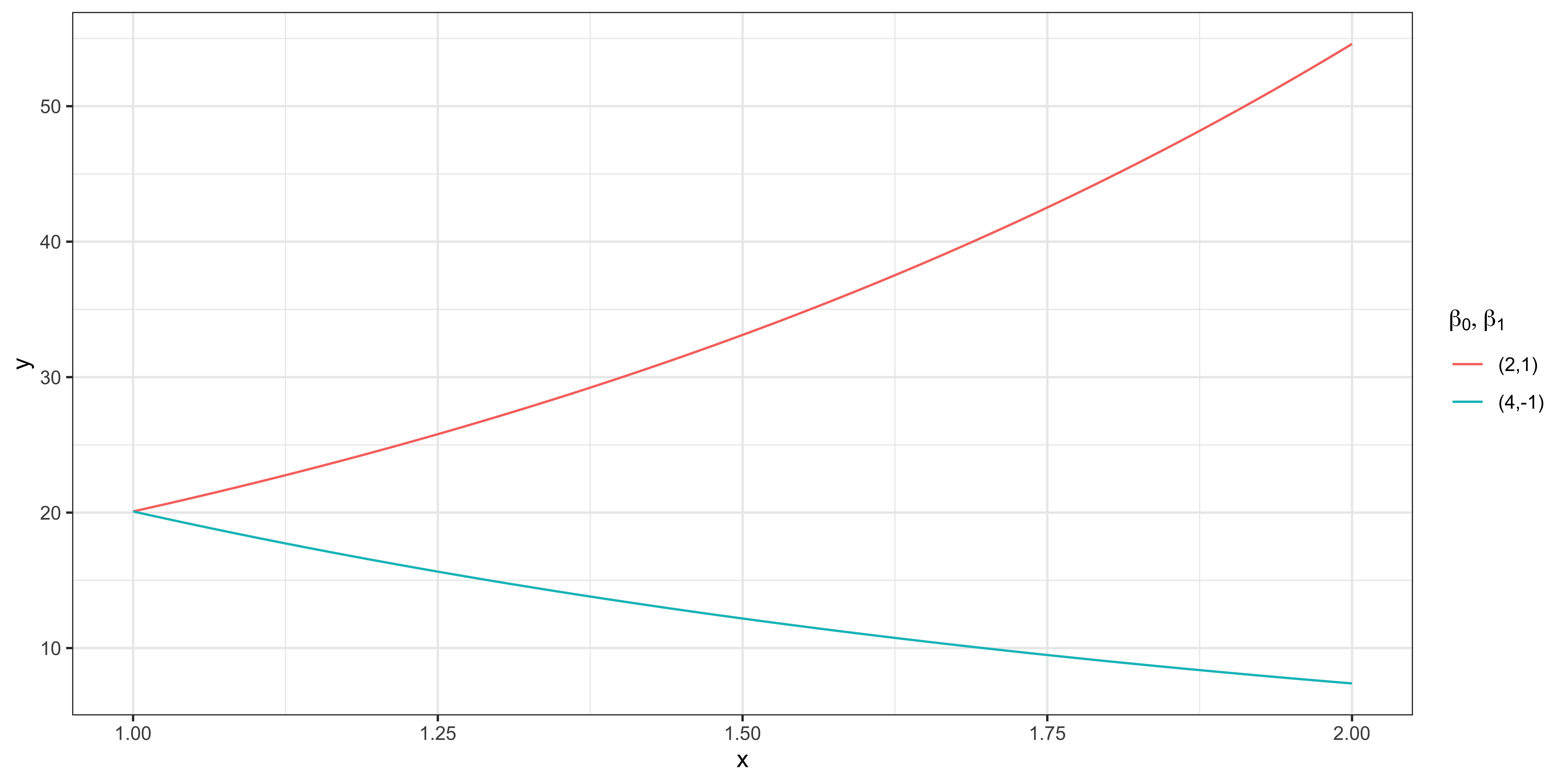
This figure translates the log-linear equation back into the original units of y. The horizontal axis is x, running from one to two, and the vertical axis is y. The legend labels each curve by the pair beta zero, beta one. The curve associated with two comma one uses y equals exponential of two plus x. The curve associated with four comma negative one uses y equals exponential of four minus x.

Why exponential? Starting from log y equals beta zero plus beta one x, exponentiate both sides. Ignoring the disturbance for the moment, y equals exponential of beta zero plus beta one x. That is why a model that is linear in log y becomes curved when we plot y itself. For the positive beta one curve, y rises as x rises, and the increase becomes steeper because the marginal effect in levels is beta one times y. A larger current y produces a larger absolute change. For the negative beta one curve, y falls as x rises and approaches zero from above.

The graph illustrates two restrictions. First, the sign of beta one determines whether the curve always rises or always falls; this simple form cannot turn around. Second, the fitted level is always positive because an exponential is positive. That can be substantively appealing for wages, prices, or yields, which should not have negative fitted values. A level-on-level straight line has no such protection when extrapolated. Do not confuse positivity with realism, however. The exponential shape is still a strong assumption. Flip to the example tab to see how the percentage interpretation is used for wages.

Transcript

Now apply the general log-linear derivation to a familiar labor-economics model. The first line says log wage equals beta zero plus beta one times education plus u. Wage is the hourly wage in positive level units, and education is measured in years. Beta zero is the fitted log wage at zero years of education, which may not be the quantity we care most about. Beta one is the slope of log wage with respect to education.

The calculus line makes that interpretation explicit. Differentiating log wage with respect to education gives one over wage times partial wage over partial education on the left and beta one on the right. For a small change, delta wage over wage is approximately beta one times delta education. If education rises by one year, delta education equals one, so the proportional wage change is approximately beta one. Multiplying by one hundred converts that proportion to a percentage. Thus we say that one additional year of education is associated with an approximately one hundred beta one percent change in hourly wage, holding the other included regressors fixed.

Use “associated with” unless the assumptions needed for a causal return are justified. Education may be correlated with ability, family background, or other determinants in u, so the functional form alone does not solve omitted-variable bias. The log specification changes the scale and interpretation, not identification. Its percentage effect is nevertheless useful because it is comparable across workers with different wage levels and across settings with different currencies or price levels. For a non-small beta one, remember the exact one-year percentage is one hundred times exponential beta one minus one. On the next tab we estimate the model and compare its curved level prediction with a straight-line wage regression.

Model

\begin{align*} log(wage)=\beta_0 + \beta_1 educ + u \notag \end{align*}

Calculus

Differentiating both sides with respect to educ,

\begin{align*} \frac{1}{wage} \frac{\partial wage}{\partial educ} = \beta_1 \Rightarrow \frac{\Delta wage}{wage} = \beta_1\Delta educ\notag \end{align*}

Interpretation

If education increases by 1 year (\Delta educ=1), then wage increases by \beta_1*100\% (\frac{\Delta wage}{wage}=\beta_1)

Transcript

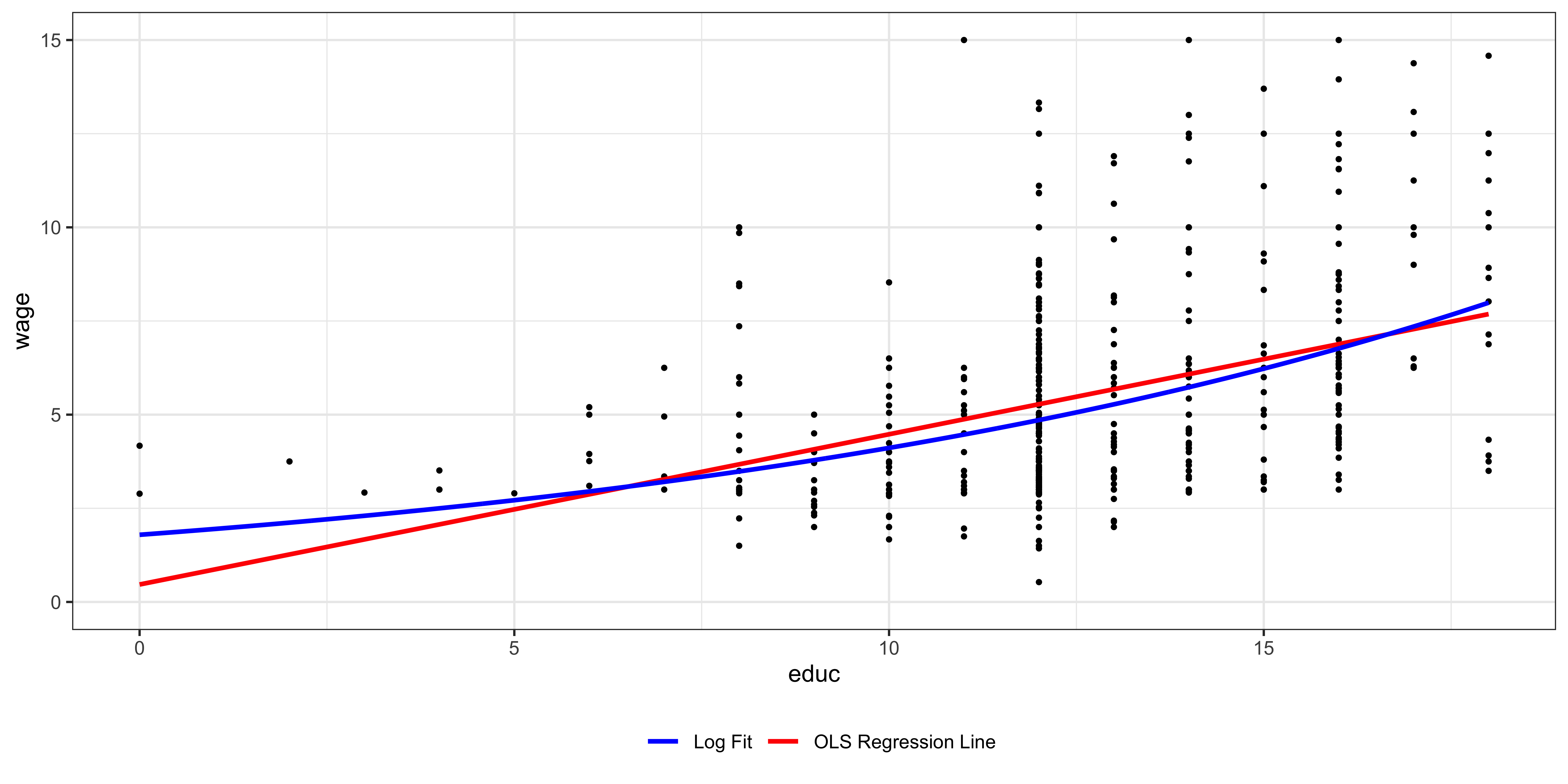
The left side gives the estimated log-linear model. The first fitted equation says predicted log wage equals zero point five eight four plus zero point zero eight three times education. The slope means that one additional year of education is associated with approximately an eight point three percent higher wage. Using the exact calculation gives one hundred times exponential of zero point zero eight three minus one, which is about eight point seven percent. The second equation exponentiates the fitted log value, producing exponential of zero point five eight four plus zero point zero eight three education in wage units.

Now look at the figure. The horizontal axis is years of education and the vertical axis is hourly wage, limited on screen to zero through fifteen dollars. Each dot is an observation from the wage data. The red “OLS Regression Line” comes from regressing wage in levels directly on education, so it is straight. The blue “Log Fit” is the exponentiated log-linear prediction, so it curves upward. The two fits can be similar near the center of the education distribution but diverge near the ends because one imposes a constant dollar slope and the other imposes a constant proportional slope. The sparse endpoints also remind you to be cautious about extrapolating either fit.

The callout is essential. If log wage equals its fitted value plus u, exponentiating gives wage equals exponential of the fitted value times exponential u. Simply exponentiating the fitted line omits the conditional mean of exponential u. Under a symmetric log error, the fitted log line corresponds to the conditional median of wage, not generally its conditional mean. Jensen’s inequality gives expected exponential u greater than exponential of expected u, so recovering the mean requires a retransformation factor, such as a distributional correction or a smearing estimate. The slide deliberately labels the plotted blue curve as the exponentiated fit, not an automatically unbiased mean prediction.

When you estimate the following model using the wage dataset:

log(wage)=\beta_0 + \beta_1 educ + u \notag


Then, the estimated equation is the following:

\begin{align*} \widehat{log(wage)}=0.584+0.083 educ \notag \end{align*} \begin{align*} \widehat{wage}=e^{0.584+0.083 educ} \end{align*}
Careful

Exponentiating the fitted line gives the predicted median of wage, not its mean. Because E[e^u]>e^{E[u]}, recovering E[wage\mid educ] requires an extra retransformation factor.

Transcript

In the linear-log model, y remains in its original units and only x is logged. The model line reads y sub i equals beta zero plus beta one times log x sub i plus u sub i. Because log x appears, x must be positive. Beta zero is the fitted value when log x is zero, which means x equals one, not when x equals zero.

Follow the calculus line carefully. The derivative of y with respect to x is the quantity we want. The derivative of beta one log x is beta one divided by x, so partial y over partial x equals beta one over x. For a small finite change, multiply by delta x: delta y is approximately beta one times delta x over x. The fraction delta x over x is a proportional change in x.

This produces a level response to a percentage change. If x rises by one percent, delta x over x is zero point zero one, and y changes by approximately zero point zero one times beta one units of y. Do not say y changes by beta one percent. Y is not logged, so its change is measured in y’s original units. Do not say a one-unit increase in x changes y by beta one either. The one-unit marginal effect is beta one over the current x and therefore varies with x.

That dependence creates diminishing absolute effects when beta one is positive: the same one-unit increase in x matters more when x is small than when x is large. Yet the effect of a fixed percentage increase is constant. This form is useful for variables such as income, acreage, or firm size when proportional changes in x are economically natural. The visualization tab shows the resulting shape and helps distinguish it from a quadratic.

Model

\begin{align*} y_i= \beta_0+\beta_1 log(x_i) +u_i \notag \end{align*}

Calculus

Differentiating the both sides wrt x_i,

\begin{align*} \frac{\partial y_i}{\partial x_i} = \frac{\beta_1}{x_i} \Rightarrow \Delta y_i = \beta_1\frac{\Delta x_i}{x_i} \notag \end{align*}

Interpretation

When x increases by 1\% (that is, \frac{\Delta x_i}{x_i} = 0.01), y increases by \beta_1 \times 0.01 units.

Transcript

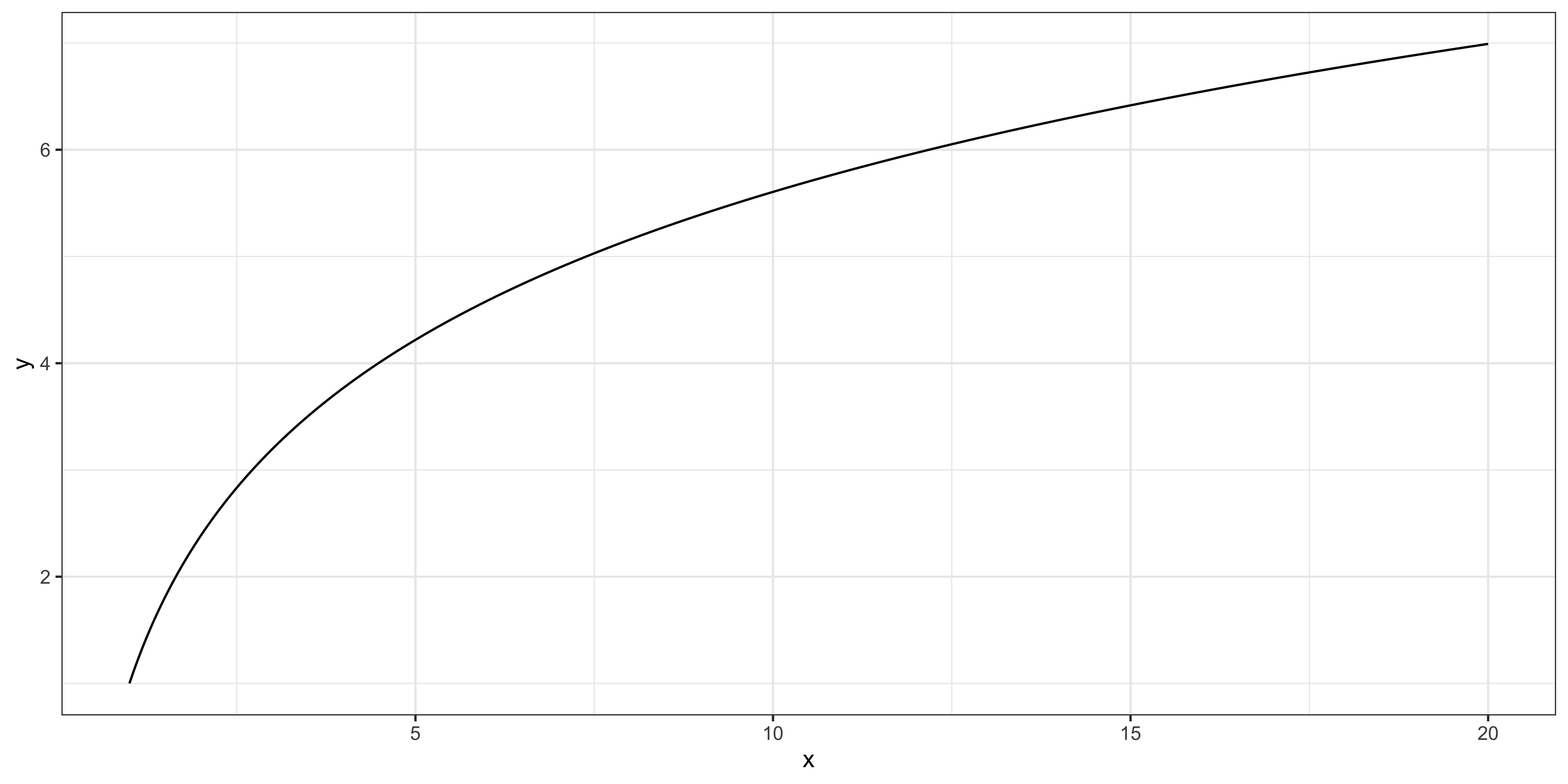
The equation above the plot fixes beta zero at one and beta one at two, so the curve is y equals one plus two times log x. The horizontal axis is x, shown from one to twenty, and the vertical axis is y in level units. At x equal to one, log one is zero, so the curve begins at y equal to one. As x rises, y rises, but the line becomes progressively flatter.

The derivative explains that shape. Partial y over partial x equals two over x. At x equal to one, the slope is two. At x equal to ten, it is zero point two. At x equal to twenty, it is zero point one. Thus equal one-unit increases in x have smaller effects at larger starting values. By contrast, equal percentage increases have the same effect on y because beta one multiplies the proportional change in x.

This graph also shows what the linear-log form cannot do. With positive beta one it is always increasing over positive x, although at a diminishing rate. It never reaches a peak and turns downward. With negative beta one it would always decrease, with the absolute slope becoming smaller as x rises. A quadratic can turn because its marginal effect is linear in x and can cross zero. Choosing between these forms therefore encodes a substantive restriction. Use linear-log if theory suggests diminishing effects that retain the same sign; use a quadratic if a reversal is plausible. Also remember the domain restriction: the log is undefined at zero and for negative x, so this specification cannot be used mechanically for every regressor.

y = \beta_0 + \beta_1 log(x) = 1 + 2 \times log(x)
Transcript

In the log-log model, both the dependent variable and the regressor are transformed. The first equation reads log y sub i equals beta zero plus beta one times log x sub i plus u sub i. Both x and y must therefore be positive.

The calculus line is written as a ratio of proportional derivatives. Differentiating gives one over y times partial y over partial x equals beta one times one over x. Rearranging, the percentage change in y divided by the percentage change in x equals beta one. In finite-change language, delta y over y is approximately beta one times delta x over x. If x rises by one percent, y changes by approximately beta one percent. A negative beta one means the variables move in opposite directions, as in a downward-sloping demand curve; a positive beta one means they move together.

Beta one is therefore an elasticity. It is unit-free, so measuring x in dollars or cents and y in pounds or kilograms does not change it. That makes the specification especially common in demand, supply, and production models. The phrase “constant elasticity” on the slide is a restriction, not merely a convenient interpretation. The model requires the same percentage response at every positive value of x. In level form, ignoring u, y equals exponential beta zero times x raised to beta one, so the absolute slope can change even though the elasticity remains fixed.

Be precise about the approximation. For a small percentage change, beta one times that percentage is accurate. For a large discrete change, use the exact log-change relationship or compare fitted levels rather than treating the differential as exact. If theory says elasticity itself varies with price, income, or scale, this simple log-log model cannot capture that variation without additional terms. We now turn to a quadratic, where the marginal effect is explicitly allowed to change with x.

Model

\begin{align*} log(y_i)= \beta_0+\beta_1 log(x_i) +u_i \notag \end{align*}

Calculus

Differentiating the both sides wrt x_i,

\begin{align*} \frac{\partial y_i}{y_i}/\frac{\partial x_i}{x_i} = \beta_1 \Rightarrow \frac{\Delta y_i}{y_i} = \beta_1 \frac{\Delta x_i}{x_i}\notag \end{align*}

Interpretation

A percentage change in x would result in a \beta_1 percentage change in y_i (constant elasticity)

Transcript

The quadratic model adds x squared as a second regressor: y sub i equals beta zero plus beta one x sub i plus beta two x sub i squared plus u sub i. It is curved in x but still linear in the parameters because beta one and beta two simply multiply two known columns, x and x squared.

Look at the calculus line. Differentiate term by term with respect to x. Beta zero disappears, beta one x contributes beta one, and beta two x squared contributes two beta two x. The marginal effect is therefore beta one plus two times beta two times x. For a one-unit increase in x, the small-change approximation says y changes by that expression, evaluated at the starting value of x.

This dependence on x is the central feature. There is no single constant effect of x to report. Beta one alone is the marginal effect only at x equal to zero. If zero is outside the observed data or has no meaningful interpretation, treating beta one as “the effect of x” is misleading. Beta two controls how the slope changes: each one-unit increase in x changes the marginal effect by two beta two. A positive beta two makes the slope increase with x; a negative beta two makes it decrease.

Because both coefficients enter the marginal effect, inference at a particular x generally concerns a linear combination of beta one and beta two. The individual t-statistics do not answer whether that combination is zero. We will return to that point in the significance section. First, the next tabs show the range of shapes a quadratic can produce and apply it to returns to education.

Model

y_i= \beta_0 + \beta_1 x_i + \beta_2 x_i^2 + u_i


Calculus

Differentiating the both sides wrt x_i,

\frac{\partial y_i}{\partial x_i} = \beta_1 + 2*\beta_2 x_i\Rightarrow \Delta y_i = (\beta_1 + 2*\beta_2 x_i)\Delta x_i


Interpretation

When x increases by 1 unit (\Delta x_i=1), y increases by \beta_1 + 2*\beta_2 x_i

Transcript

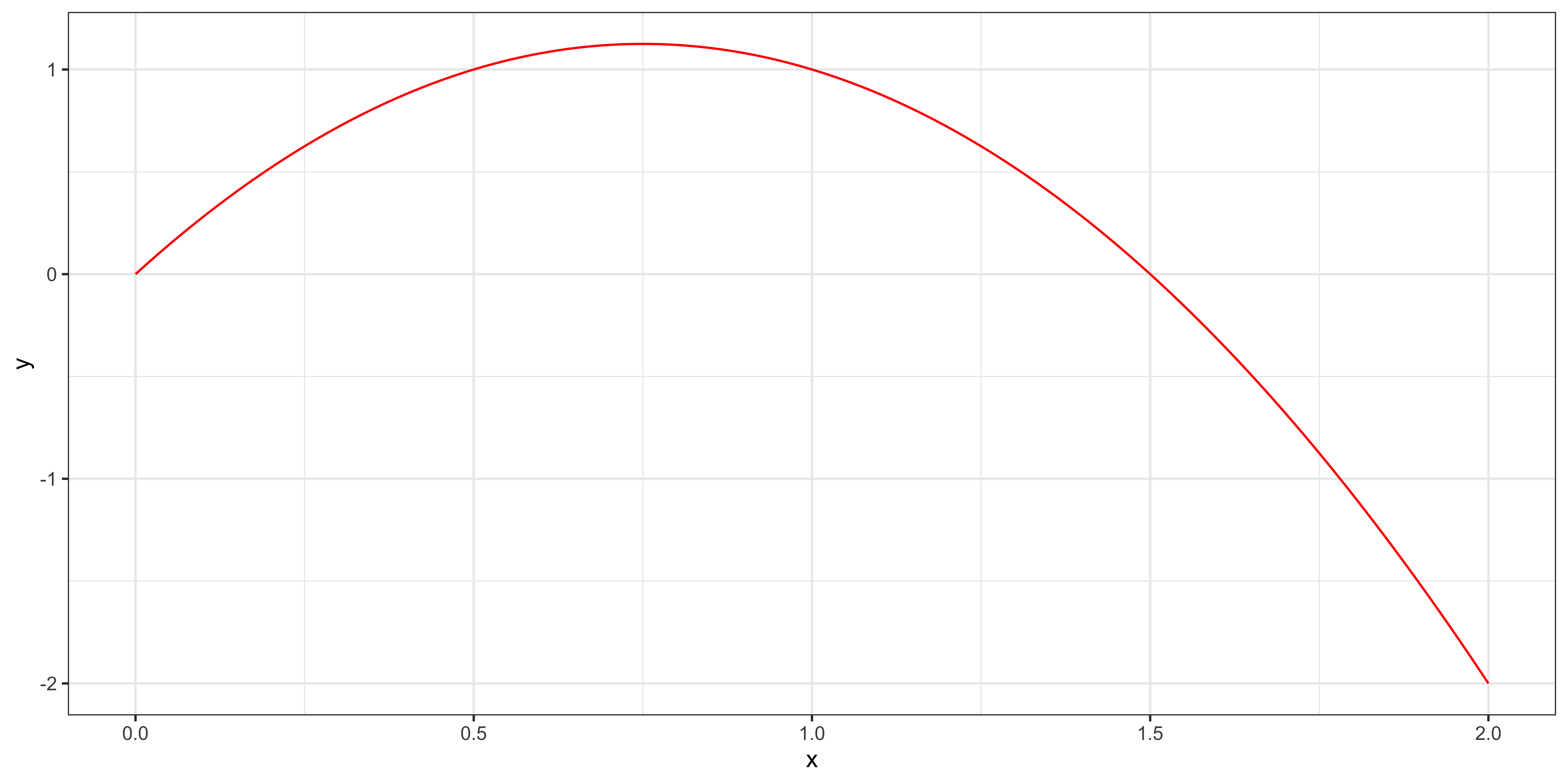
These two panels plot quadratic functions over x from zero to two. In both panels, the horizontal axis is x and the vertical axis is y. The left equation is y equals x plus x squared, so beta one and beta two both equal one. Its marginal effect is one plus two x, which is positive and increasing throughout the plotted range. The curve therefore rises and becomes steeper as x increases.

The right equation is y equals three x minus two x squared. Here beta one is three and beta two is negative two. Its marginal effect is three minus four x. At x equal to zero the slope is three; it falls as x increases, reaches zero at x equal to three quarters, and becomes negative after that. The red curve consequently rises, peaks, and then falls. In general, a quadratic turning point occurs where beta one plus two beta two x equals zero, so x star is minus beta one divided by two beta two. When beta two is negative, that point is a maximum; when beta two is positive, it is a minimum.

This is why the slide calls the form flexible. It can represent increasing returns, diminishing returns, a peak, or a trough. But it always imposes a parabola, and its behavior can become extreme outside the data. Before discussing a turning point, calculate it and compare it with the observed support of x. If it lies outside that support, the estimated relationship may simply be increasing or decreasing over the relevant range. Do not claim that the outcome eventually reverses based on an extrapolated part of the parabola. The education example on the next tab shows why a changing slope can be economically plausible.

Quadratic functional form is quite flexible.

y = x + x^2 (\beta_1 = 1, \beta_2 = 1)
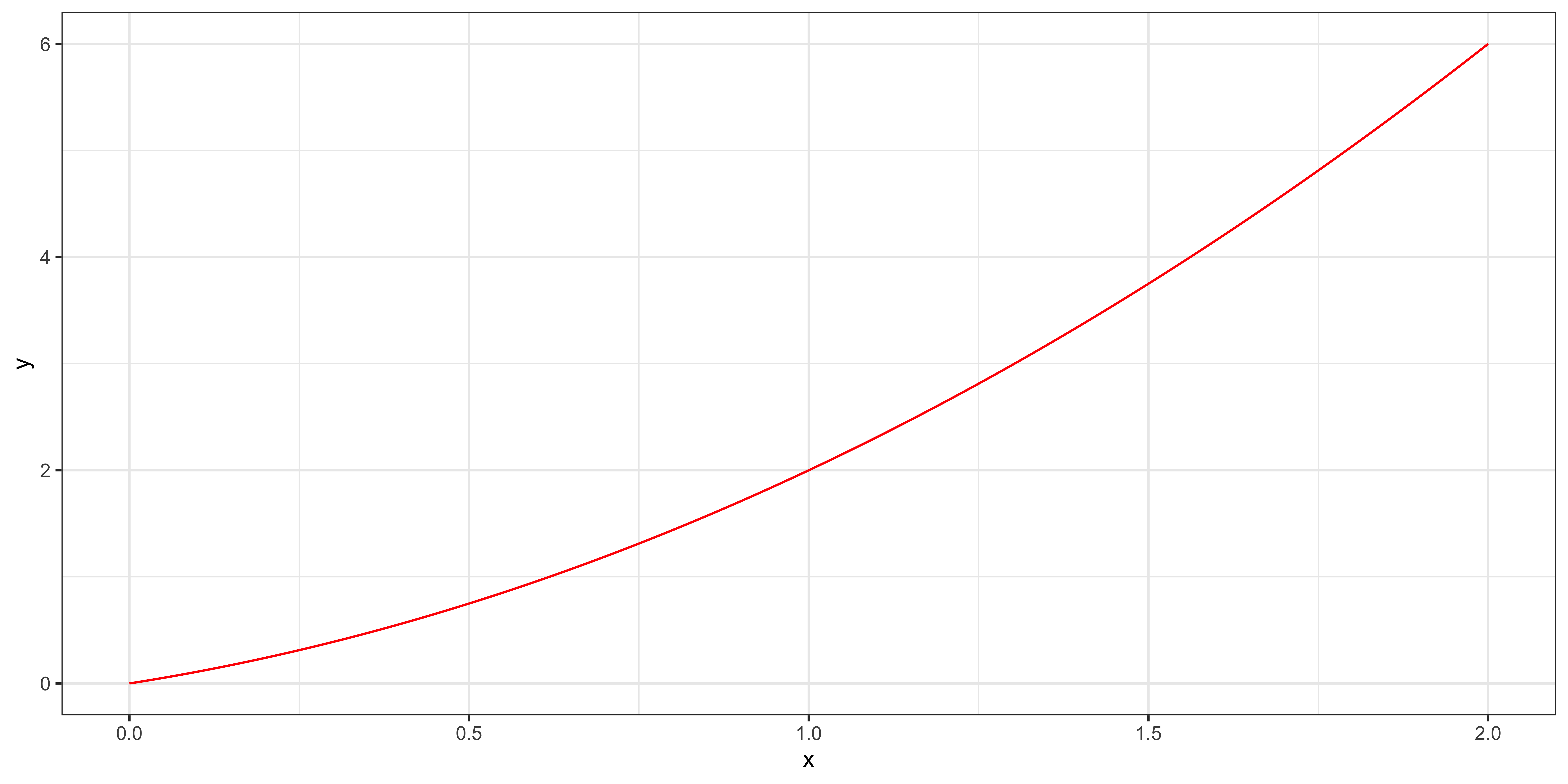
y = 3x-2x^2 (\beta_1 = 3, \beta_2 = -2)
Transcript

Use the three questions to see why a constant return to education may be too restrictive. The outcome of interest is income or wage, and the marginal impact of education means the change in expected income associated with a small increase in years of schooling, holding the other modeled factors fixed.

The first bullet asks about adding two years after elementary school. Those years might move a person toward completing a credential or acquiring foundational skills. The second asks about two years after college, perhaps a master’s degree or professional training. The third asks about adding two years after already spending six years in a doctoral program. Those increments all have the same numerical size, two years, but there is no strong reason to assume that the labor market values them identically. Credentials, field, opportunity cost, and the changing scarcity of skills can all make the return depend on the starting education level.

A model with only one education term forces all three cases to share the same slope. That equality comes from the specification, not from evidence. The observation at the bottom says the marginal impact does not appear to be linear, meaning more precisely that the level relationship may not have a constant marginal effect. Adding education squared is the simplest way to let the slope change smoothly with education. In that model the marginal effect is beta education plus two times beta education squared times education, so we can evaluate the return at elementary-school, college, or doctoral levels separately. This does not guarantee that a quadratic is correct, and it does not establish a causal effect. It is a transparent first relaxation of the constant-slope assumption. The next tab shows how to estimate it in R.

Education impacts on income

The marginal impact of education (the impact of a small change in education on income) may differ depending on the level of education you have had:

  • How much does it help to have two more years of education when you have had education until elementary school?

  • How much does it help to have two more years of education when you have graduated a college?

  • How much does it help to spend two more years as a Ph.D student if you have already spent six years in a Ph.D program


Observation

The marginal impact of education does not seem to be linear.

Transcript

The sentence above the code gives the formula rule to remember. Inside an R model formula, operators can have special formula meanings, so wrap literal arithmetic in capital I. Here I of education caret two tells R to calculate education squared observation by observation and include that numeric column. Without I, the caret is interpreted by the formula language rather than simply as the arithmetic square you intend.

The runnable regression call is fixest colon colon feols. Its first argument specifies wage as the dependent variable and includes female, education, and I of education squared on the right. Female controls for the average level difference associated with the binary indicator. The two education terms together create the quadratic. The vcov argument is set to “hetero,” asking fixest for heteroskedasticity-robust standard errors. The data argument points to wage1, which the preceding data call loads from the wooldridge package. Assigning the result to quad_reg lets later tabs reuse the same fitted model. Finally, broom colon colon tidy converts the model output into one row per coefficient with the estimate, standard error, test statistic, and p-value.

When you run the cell, the fitted education coefficient is about negative zero point four one six and the coefficient on education squared is about positive zero point zero three nine five. Those signs imply a U-shaped fitted parabola, and the marginal effect is negative zero point four one six plus two times zero point zero three nine five times education. Do not interpret the negative coefficient on education alone as education generally reducing wage. It is the slope at education equal to zero. The combination of both coefficients determines the slope at every education level. The setup code above prepares the WebR plotting theme and packages for the browser; it does not change the econometric specification. The next tab plots the fitted relationship so you can judge it against the observations.

When you want to include a variable that is a transformation of an existing variable, you can use I() function in which you write the mathematical expression of the desired transformation.

Transcript

The displayed fitted equation summarizes the quadratic regression: wage equals about five point six zero, minus two point one two times female, minus zero point four one six times education, plus zero point zero three nine times education squared. The intercept is the fitted wage for a man, because female equals zero, at zero years of education. The female coefficient shifts the fitted curve downward when female equals one. The final two terms determine how the curve changes with schooling.

Now read the plotting code and figure. The sequence x runs from the minimum to the maximum education observed in wage1. The new data table sets education equal to each value in that sequence and female equal to one, so the plotted line is specifically the fitted relationship for women. Predict with newdata calculates the model’s fitted wage at each of those combinations. In the graph, the horizontal axis is education in years and the vertical axis is hourly wage. The points are the observed wage and education pairs for everyone in the sample, while the line is the female-equals-one prediction. Because the points include both women and men but the line is for women, use the scatter mainly to see support and overall fit, not as a within-group residual display.

The line falls slightly at very low education and then rises increasingly steeply. Its turning point solves negative zero point four one six plus two times zero point zero three nine five times education equals zero, which is about five point three years. Very few observations lie at the lowest schooling levels, so the apparent decline rests on sparse support and the imposed parabolic shape. The safe conclusion is that the fitted marginal effect becomes more positive as education increases over the well-populated part of the sample. Always overlay or otherwise inspect the data before interpreting a quadratic’s turning point, especially near a boundary.

Estimated Model

wage = 5.60 - 2.12\times female -0.416\times educ + 0.039\times educ^2

Transcript

Start with the fitted equation from the previous tab and differentiate it with respect to education. The constant and female terms disappear. The derivative of negative zero point four one six times education is negative zero point four one six, and the derivative of zero point zero three nine times education squared is two times zero point zero three nine times education. That gives the displayed marginal effect: negative zero point four one six plus zero point zero seven eight times education, measured in dollars of hourly wage per additional year of schooling.

Evaluate the expression at the two values shown. At education equal to four, the fitted marginal effect is negative zero point four one six plus zero point zero seven eight times four, about negative zero point one zero four dollars per hour for an additional year. At education equal to ten, it is negative zero point four one six plus zero point zero seven eight times ten, about positive zero point three six four dollars per hour. The sign changes because the quadratic slope rises with education. These are local marginal effects, not the exact fitted change from four to five or ten to eleven; for a discrete one-year change, the squared term also contributes beta education squared times one squared. The derivative is the standard marginal-effect summary.

The next issue is uncertainty. The marginal effect at a chosen education level combines the estimated linear and squared coefficients. Its variance includes the variance of each estimate and their covariance. Neither individual t-statistic answers whether this combination differs from zero. The education t-test concerns the slope only at zero education, and the squared-term t-test concerns curvature. We need a test of one linear restriction at each education level. That is the purpose of the next section.

According to the estimated model, the marginal impact of educ is:

\frac{\partial wage}{\partial educ} = -0.416+0.039\times 2\times educ

  • When educ = 4, additional year of education is going to increase hourly wage by -0.104 on average

  • When educ = 10, additional year of education is going to increase hourly wage by 0.364 on average

Statistical significance of the marginal impact


Statistical significance of the marginal impact

Transcript

This slide turns the quadratic marginal effect into an inference question. The expression at the top is negative zero point four one six plus two times zero point zero three nine times education. The first number estimates the coefficient on education, and the second estimates the coefficient on education squared. Because education appears in the weight on the squared-term coefficient, the estimated marginal effect changes with the education level at which you evaluate it.

The two bullets report the individual coefficients and their t-statistics. Be clear about what those separate tests ask. The t-test on beta education asks whether the coefficient on the linear education term is zero. In a quadratic model, that coefficient is the marginal effect only at education equal to zero. The t-test on beta education squared asks whether there is curvature, meaning whether the marginal effect changes with education. Neither test directly asks whether the marginal effect is zero at four, ten, or any other nonzero level.

At a chosen value c, the parameter of interest is beta education plus two c times beta education squared. Its estimated variance is the variance of beta hat education, plus four c squared times the variance of beta hat education squared, plus four c times the covariance between the two coefficient estimates. That covariance matters because both estimates came from the same regression. The standard error is the square root of that full variance, not the sum of the two printed standard errors.

So the question at the bottom, “is the marginal impact statistically significantly different from zero,” is incomplete until we specify education. A quadratic can yield an effect that is indistinguishable from zero at one schooling level and clearly positive at another. We will first revisit the linear case, where the effect is one coefficient and the usual output suffices, then build the appropriate linear-combination test for the quadratic case.

Let’s work with the income model, in which the marginal impact of educ is:

\begin{align*} \frac{\partial wage}{\partial educ} = -0.416+0.039\times 2\times educ \end{align*}
  • \beta_{educ}: -0.416 (t-stat = -1.80)
  • \beta_{educ^2}: 0.039 (t-stat = 4.10)


Question

So, is the marginal impact of educ statistically significantly different from 0?

Transcript

Start with the linear specification as a benchmark. The code calls fixest colon colon feols with wage on the left and female plus education on the right. The data argument uses wage1. The vcov argument requests heteroskedasticity-robust standard errors, so the uncertainty calculation does not assume a constant error variance. Broom tidy prints the intercept, female coefficient, and education coefficient with their robust standard errors, test statistics, and p-values. Autorun means the browser evaluates the cell automatically when it is ready.

The estimated equation below the output is wage equals zero point six two, minus two point two seven times female, plus zero point five one times education. Holding education fixed, the female coefficient is the fitted wage difference between observations coded one and the male baseline coded zero. Holding female fixed, one additional year of education is associated with about zero point five one dollars more in hourly wage.

Differentiate this linear equation with respect to education. The derivative is simply beta education, estimated at about zero point five zero six. It contains no education value, so the model imposes the same marginal effect at four, ten, and eighteen years. That constancy is what makes inference easy: the null that the marginal effect is zero is exactly the null that beta education is zero. The regression output’s education t-statistic, about eight point four six with a p-value far below one percent, answers it directly. Work through both question tabs because they separate a result from an assumption: zero point five one is the fitted effect, while its constancy was imposed by choosing a linear functional form.

Regression


Estimated model

wage = 0.62 - 2.27 \times female + 0.51 \times educ


Transcript

Question one asks for the marginal impact of education in the fitted linear model. Look at the equation immediately above this tab: wage equals zero point six two, minus two point two seven times female, plus zero point five one times education. Differentiate with respect to education. The intercept and female term do not change, and the derivative of zero point five one times education is zero point five one.

So the answer is about zero point five one dollars of hourly wage per additional year of education, holding female fixed. The units are important. Wage is in dollars per hour and education is in years, so this is not a percentage and not five point one percent. It is also an association conditional on the included dummy, unless the model’s exogeneity assumptions justify causal language.

The answer is simple only because education enters once and linearly. There is no squared term, log, or interaction that would add another coefficient or make the derivative depend on another variable. Keep that special structure in mind when you move to question two.

What is the marginal impact of educ?


Answer 0.51
Transcript

Question two asks whether the marginal impact varies with the level of education. In this fitted equation the answer is no. The derivative with respect to education is the constant coefficient zero point five one, and education itself does not appear in that derivative. The model therefore assigns the same fitted increase in hourly wage to an extra year after eight years of schooling as to an extra year after eighteen.

Notice what kind of statement this is. We did not use the data to test whether those two marginal effects are equal. We made them equal by writing a model with only one linear education term. A straight-line specification has a constant slope by construction. The answer panel correctly says the model assumed the marginal impact is constant.

That distinction matters whenever you interpret a regression. A restriction implied by functional form is not an empirical finding. If economic reasoning suggests that returns vary with schooling, add a term that allows such variation, such as education squared or an interaction with a degree category, and then estimate and test it. In the quadratic case the derivative contains both education and education squared coefficients, so the answer changes with the evaluation point. Flip to the testing tab first to finish the easy linear case.

Does the marginal impact of education vary depending on the level of education?


Answer No, the model we estimated assumed that the marginal impact of education is constant.
Transcript

In the linear model, the marginal effect of education is beta education itself. To ask whether education has a nonzero marginal impact, write the null as beta education equals zero and the two-sided alternative as beta education does not equal zero. That is a restriction on one population coefficient, so it is the ordinary t-test printed on the education row of the regression table.

The t-statistic is beta hat education minus the null value zero, divided by the standard error of beta hat education. Its sign tells you the estimated direction, and its magnitude tells you how many standard errors the estimate lies from zero. The p-value measures how surprising a statistic at least that extreme would be under the null. In the output from the model tab, the robust t-statistic is about eight point four six and the p-value is essentially zero at conventional display precision, so we reject the null.

Nothing extra is required because the parameter of interest and one reported coefficient are the same object. This convenience disappears when a derivative contains two or more coefficients. Then you need the estimate and standard error of the whole linear combination, including covariances among estimates. The quadratic tabs show how to do that without manually constructing the covariance calculation.

You can just test if \hat{\beta}_{educ} (the marginal impact of education) is statistically significantly different from 0, which is just a t-test.

Transcript

The three bullets summarize what changes in the quadratic specification. First, the marginal impact of education depends on the current education level because the derivative is beta education plus two times beta education squared times education. Two people at different schooling levels generally have different fitted slopes even though they are evaluated using the same estimated model.

Second, there is no single test of “the marginal effect” that applies universally. A test at education equal to four concerns beta education plus eight beta education squared. A test at education equal to ten concerns beta education plus twenty beta education squared. Those are different population quantities and have different estimates and standard errors. Rejecting one null does not logically imply rejecting the other.

Third, you need to choose evaluation levels and test the relevant combination at each one. That choice should come from the research question and the support of the data. Useful values may correspond to meaningful schooling milestones or selected quantiles of the observed distribution. Avoid reporting effects at levels with few or no observations, and avoid searching across many values merely to find significance. If you want to summarize the effect over a range, you can report several prespecified points or a marginal-effect curve with a confidence band.

Also distinguish these pointwise tests from a test that education plays no role anywhere. A joint null that both the linear and squared education coefficients are zero asks whether the two education terms are jointly irrelevant. That is not the same as asking whether the derivative equals zero at one chosen level. The next tab starts with education equal to four and constructs exactly one linear restriction.

With the quadratic specification

  • The marginal impact of education varies depending on your education level

  • There is no single test that tells you whether the marginal impact of education is statistically significant universally

  • Indeed, you need different tests for different education levels

Transcript

The research question here is local and two-sided: for a person currently at four years of education, does one additional year have a positive or negative marginal impact that differs from zero? Begin with the derivative beta education plus two times beta education squared times education. Substituting four gives beta education plus eight beta education squared.

The null is therefore beta education plus eight beta education squared equals zero, and the alternative says that same combination does not equal zero. The callout emphasizes that hypotheses concern the population parameters beta, without hats. We do not hypothesize that the random estimates equal zero. We use the estimates to form evidence about the unknown population combination.

Now answer the multiple-choice prompt. This is not a test of one coefficient because two coefficients appear. It is also not a test of multiple equations. It is one equation, or one linear restriction, involving multiple coefficients. A single restriction can be tested with a t-statistic. An equivalent one-restriction F-statistic is the square of that t-statistic when both use the same variance estimate and denominator degrees of freedom.

Look at the t formula. The numerator is beta hat education plus eight beta hat education squared, the estimated marginal effect at four under a zero null. The denominator is the standard error of that whole combination. If b one and b two denote the two estimates, its variance is variance b one plus sixty-four times variance b two plus sixteen times covariance of b one and b two. That covariance is why dividing the numerator by either individual standard error would be wrong. The next tab uses software to perform this linear-restriction calculation.

Marginal impact of education

\hat{\beta}_{educ} + \hat{\beta}_{educ^2} \times 2 \times educ


Hypothesis testing

Does an additional year of education have a statistically significant impact (positive or negative) if your current education level is 4?

  • H_0: \beta_{educ} + \beta_{educ^2} \times 2 \times 4 =0

  • H_1: \beta_{educ} + \beta_{educ^2} \times 2 \times 4 \ne 0

Note

Hypotheses are statements about the population parameters \beta, never about the estimates \hat{\beta}. We use the estimates to build the test statistic below.


Question

Is this

  • test of a single coefficient? (t-test)
  • test of a single equation with multiple coefficients? (t-test)
  • test of multiple equations with multiple coefficients? (F-test)

t-statistic

t = \frac{\hat{\beta}_{educ} + \hat{\beta}_{educ^2} \times 2 \times 4}{se(\hat{\beta}_{educ} + \hat{\beta}_{educ^2} \times 2 \times 4)} = \frac{\hat{\beta}_{educ} + \hat{\beta}_{educ^2} \times 8}{se(\hat{\beta}_{educ} + \hat{\beta}_{educ^2} \times 8)}

Transcript

The car colon colon linearHypothesis function tests restrictions on coefficients from an estimated model. Its first argument is quad_reg, the quadratic wage model. Its second argument is a character string representing the null restriction. The intended string says the education coefficient plus eight times the squared-education coefficient equals zero. The coefficient names in such a string must match the names stored in the fitted model, so checking names of coef quad_reg is a good diagnostic if the function cannot parse a term.

The note above the cell explains the one-restriction equivalence. A t-test directly standardizes one estimated linear combination. An F-test for exactly one restriction squares that t-statistic, so the two-sided t-test and the one-restriction F-test give the same p-value when constructed from the same covariance estimate. With heteroskedasticity-robust covariance estimation, software may label the large-sample squared statistic as chi-squared rather than finite-sample F, but the restriction being tested is still the one displayed on the previous tab.

The slide reports a p-value of zero point three nine four. That is much larger than common significance levels such as zero point zero five, so we do not reject the null. This does not prove that the marginal effect at four is exactly zero. It says the estimate is not far enough from zero, relative to its uncertainty, to distinguish it statistically in this sample. The conclusion is specific to education equal to four. It does not tell us whether the effect is significant at ten, which is the next example.

Remember, a trick to do this test using R is take advantage of the fact that F_{1, n-k-1} \sim t_{n-k-1}^2.

The p-value is 0.394, so we do not reject the null: at an education level of 4, the marginal impact of education is not statistically distinguishable from zero.

Transcript

Now evaluate the same quadratic derivative at education equal to ten. Start with beta education plus two times beta education squared times education. Substituting ten changes the multiplier on the squared-term coefficient to twenty, so the marginal effect parameter is beta education plus twenty beta education squared.

The null says that one linear combination equals zero, and the two-sided alternative says it does not. As in example one, this is one equation involving multiple coefficients. It is therefore a single-restriction t-test, or equivalently a one-restriction F-type test. The fact that two coefficients appear does not by itself make the null a multiple-restriction hypothesis.

The t-statistic shown at the bottom divides beta hat education plus twenty beta hat education squared by the standard error of that same combination. Its variance is variance of beta hat education, plus four hundred times the variance of beta hat education squared, plus forty times their covariance. Notice how changing the evaluation point changes both the estimated marginal effect and its standard error. We are not reinterpreting the test from education equal to four. We are testing a different population quantity using the same underlying regression estimates and covariance matrix.

Numerically, using the rounded coefficients on the slide, the fitted marginal effect at ten is about negative zero point four one six plus twenty times zero point zero three nine, or positive zero point three six four dollars per hour for another year. The R implementation on the next tab determines whether that positive estimate is large relative to its uncertainty.

Marginal impact of education

\hat{\beta}_{educ} + \hat{\beta}_{educ^2} \times 2 \times educ


Hypothesis testing

Does an additional year of education have a statistically significant impact (positive or negative) if your current education level is 10?

  • H_0: \beta_{educ} + \beta_{educ^2} \times 2 \times 10 =0

  • H_1: \beta_{educ} + \beta_{educ^2} \times 2 \times 10 \ne 0

Question

Is this

  • test of a single coefficient? (t-test)
  • test of a single equation with multiple coefficients? (t-test)
  • test of multiple equations with multiple coefficients? (F-test)

t-statistic

t = \frac{\hat{\beta}_{educ} + \hat{\beta}_{educ^2} \times 2 \times 10}{se(\hat{\beta}_{educ} + \hat{\beta}_{educ^2} \times 2 \times 10)} = \frac{\hat{\beta}_{educ} + \hat{\beta}_{educ^2} \times 20}{se(\hat{\beta}_{educ} + \hat{\beta}_{educ^2} \times 20)}

Transcript

This cell uses the same linearHypothesis approach as example one, replacing the weight eight with twenty because the evaluation point is now ten years of education. The first argument remains quad_reg, so we are not re-estimating the wage equation. We are asking a new question of the same coefficient vector and covariance matrix. The character string represents the null that the education coefficient plus twenty times the squared-education coefficient equals zero.

The reported p-value is far below zero point zero one. We therefore reject the null at the one percent level and conclude that the marginal effect at ten years is statistically distinguishable from zero. The fitted combination is positive, so the estimated direction is a positive association between an additional year of education and hourly wage at that education level.

Put the two examples side by side. At four years, the p-value is zero point three nine four and we fail to reject. At ten years, the p-value is effectively zero and we reject decisively. The regression model and its estimated coefficients did not change. The evaluation point changed the linear combination being tested, and that changed both its magnitude and uncertainty. This is the practical meaning of a varying marginal effect.

Do not summarize these results by saying “education is insignificant at low levels and significant at high levels” without stating the evaluated values and acknowledging data support. These are pointwise conclusions from a quadratic model. A fuller presentation could graph the marginal effect and its confidence band over the observed education range. Next we apply the same logic to interaction terms, where one variable changes the marginal effect of another.

The p-value is far below 0.01, so we reject the null at the 1% level: at an education level of 10, the marginal impact of education is statistically significant.

Interaction terms


Interaction terms

Transcript

An interaction term is a new regressor formed by multiplying two variables. The example is education times experience. Including this product allows the marginal effect of one variable to depend on the level of the other, which a purely additive model cannot do.

Read the displayed wage model carefully. It contains an intercept, experience by itself, and education times experience. Differentiate with respect to experience and you will obtain beta one plus beta two times education, so the return to another year of experience changes with schooling. Equivalently, differentiating with respect to education gives beta two times experience, so the association with schooling changes with experience. Interaction effects are symmetric in that algebraic sense even if the research question emphasizes one direction.

The important callout warns that this is a deliberately stripped-down example. Education does not enter on its own. That omission forces education to affect wage only through experience. When experience equals zero, the fitted marginal effect of education must be exactly zero. It also makes beta one the experience slope at education equal to zero. Those are strong restrictions chosen for a short derivation, not general modeling advice.

The rule of thumb in blue is the hierarchy principle: when you include x one times x two, ordinarily include x one and x two as separate main effects too. Then each main-effect coefficient describes a slope when the other variable is zero, and the interaction coefficient describes how that slope changes. If zero is not meaningful, centering a variable can make the main effects easier to interpret without changing fitted values. Interactions are not merely extra controls. They answer questions about heterogeneity, such as whether experience is more valuable at higher education levels. The next tab derives that marginal effect explicitly.

A variable that is a multiplication of two variables


Example

educ\times exper


A model with an interaction term

wage = \beta_0 + \beta_1 exper + \beta_2 educ \times exper + u


A deliberately stripped-down model

Notice that educ does not enter on its own here. This keeps the algebra on the next slides as simple as possible, but it is not what you should do in your own work.

Rule of thumb: whenever you include an interaction x_1 \times x_2, include x_1 and x_2 as separate terms too. Omitting a main effect forces the marginal impact of exper to be exactly \beta_1 when educ = 0 and constrains educ to affect wage only through exper — a restriction you almost never want to impose.

Transcript

Start from the stripped-down model on the previous tab: wage equals beta zero plus beta one times experience plus beta two times education times experience plus u. Differentiate with respect to experience. Beta zero drops out, beta one experience contributes beta one, and beta two education experience contributes beta two times education. The marginal impact is therefore beta one plus beta two education, exactly as displayed.

The first implication follows immediately: the experience slope is not constant. Evaluate it at a particular schooling level. Beta one is the marginal effect of experience when education equals zero. That is the reference value built into the parameterization, not an overall experience effect. If nobody in the relevant population has zero education, beta one alone is an extrapolated slope and may have little substantive meaning.

Beta two tells you how much the experience slope changes when education increases by one year. Its units are dollars of hourly wage per year of experience per year of education. If beta two is positive, another year of experience is associated with a larger wage increment for people with more schooling, so the two inputs reinforce each other in the fitted model. If beta two is negative, the experience return declines with schooling.

Remember the main-effect warning. Because this teaching model omits education by itself, it also says the marginal impact of education is beta two times experience and must be zero when experience is zero. A practical hierarchical specification would usually contain female, education, experience, and their product. The interaction coefficient would still measure how the two slopes change, while the separate education term would avoid that unintended zero restriction. On the R tab we deliberately estimate the stripped-down form so its coefficients match this algebra.

Marginal impact of experience:

\frac{\partial wage}{\partial exper} = \beta_1+\beta_2\times educ


Implications

The marginal impact of experience depends on education

  • \beta_1: the marginal impact of experience when educ=0

  • if \beta_2>0: additional year of experience is worth more when you have more years of education

Transcript

The code implements the stripped-down interaction model exactly. Fixest colon colon feols estimates wage on female, experience, and the literal product of experience and education. Female is included as a level control. Experience is the main effect shown in the algebra. Capital I around experience times education tells the formula parser to perform arithmetic multiplication and create only that product column. Without I, an asterisk in an R formula expands to both main effects plus their interaction.

The assignment stores the fitted model as reg_int so later tabs can extract coefficients, make predictions, and test restrictions. There is no vcov argument in this call, so fixest reports its default IID standard errors rather than the heteroskedasticity-robust standard errors used in the quadratic example. The surrounding parentheses print the model immediately after assigning it. Autorun evaluates the cell automatically.

When run on wage1, the estimates are approximately six point one two for the intercept, negative two point four one eight for female, negative zero point one eight eight for experience, and positive zero point zero two zero four for experience times education. The interaction estimate means each additional year of education raises the fitted marginal effect of a year of experience by about two cents per hour. The negative experience coefficient is the slope at education equal to zero, so it should not be described as the experience effect for a typical worker.

For your own work, the more standard fixest formula would use education star experience, which expands to education plus experience plus their interaction. Here we retain I of the product because the previous slide intentionally omitted the education main effect. The hidden knitr chunk fits the identical model for the static figures on the next tab; it does not add another specification.

Just like the quadratic case with educ^2, you can use I().

Transcript

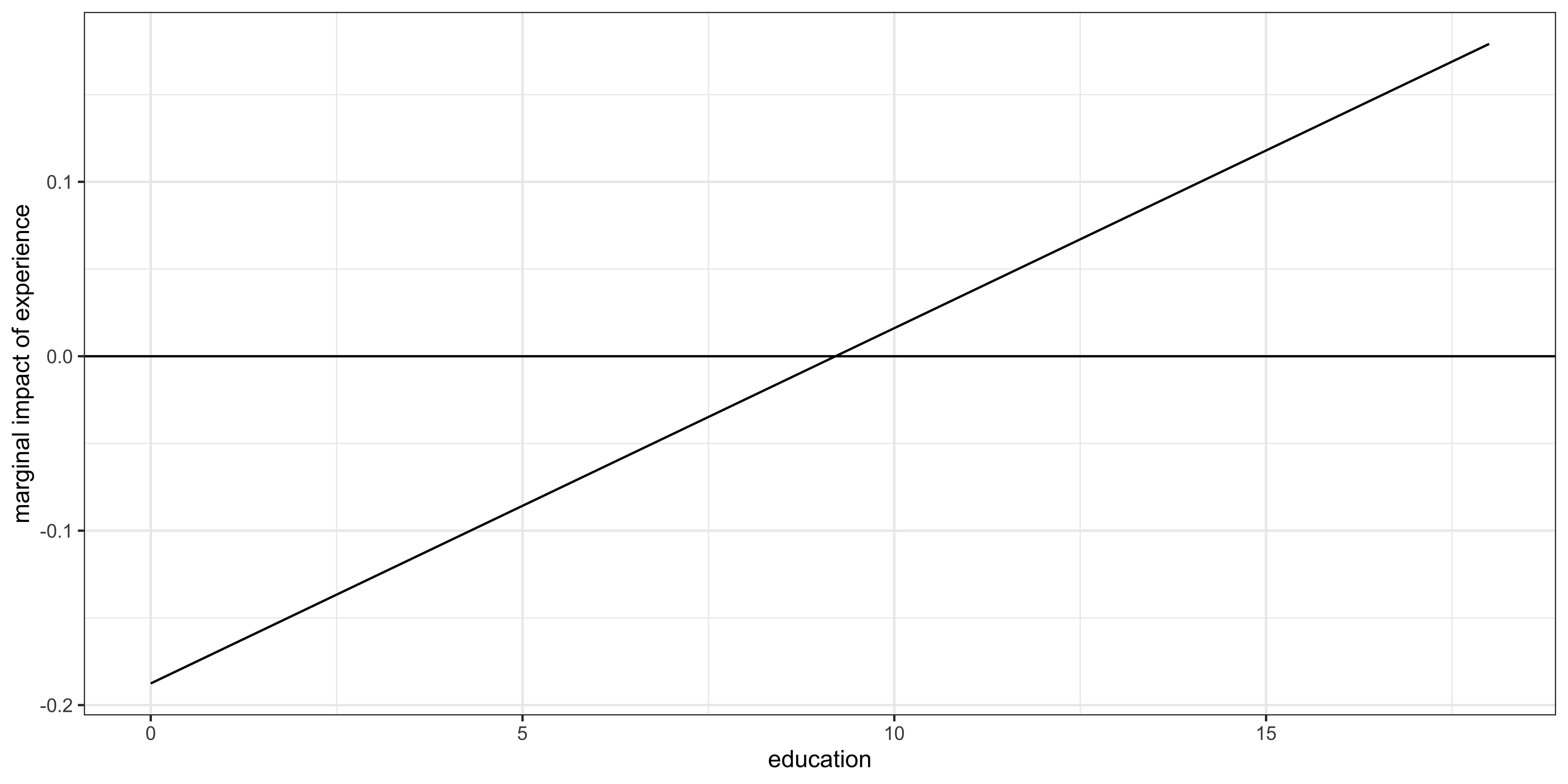
The equation at the top reports the fitted model from the previous tab. Wage equals six point one two one, minus two point four one eight times female, minus zero point one eight eight times experience, plus zero point zero two zero times education times experience. Differentiating with respect to experience gives the displayed marginal effect, negative zero point one eight eight plus zero point zero two zero times education.

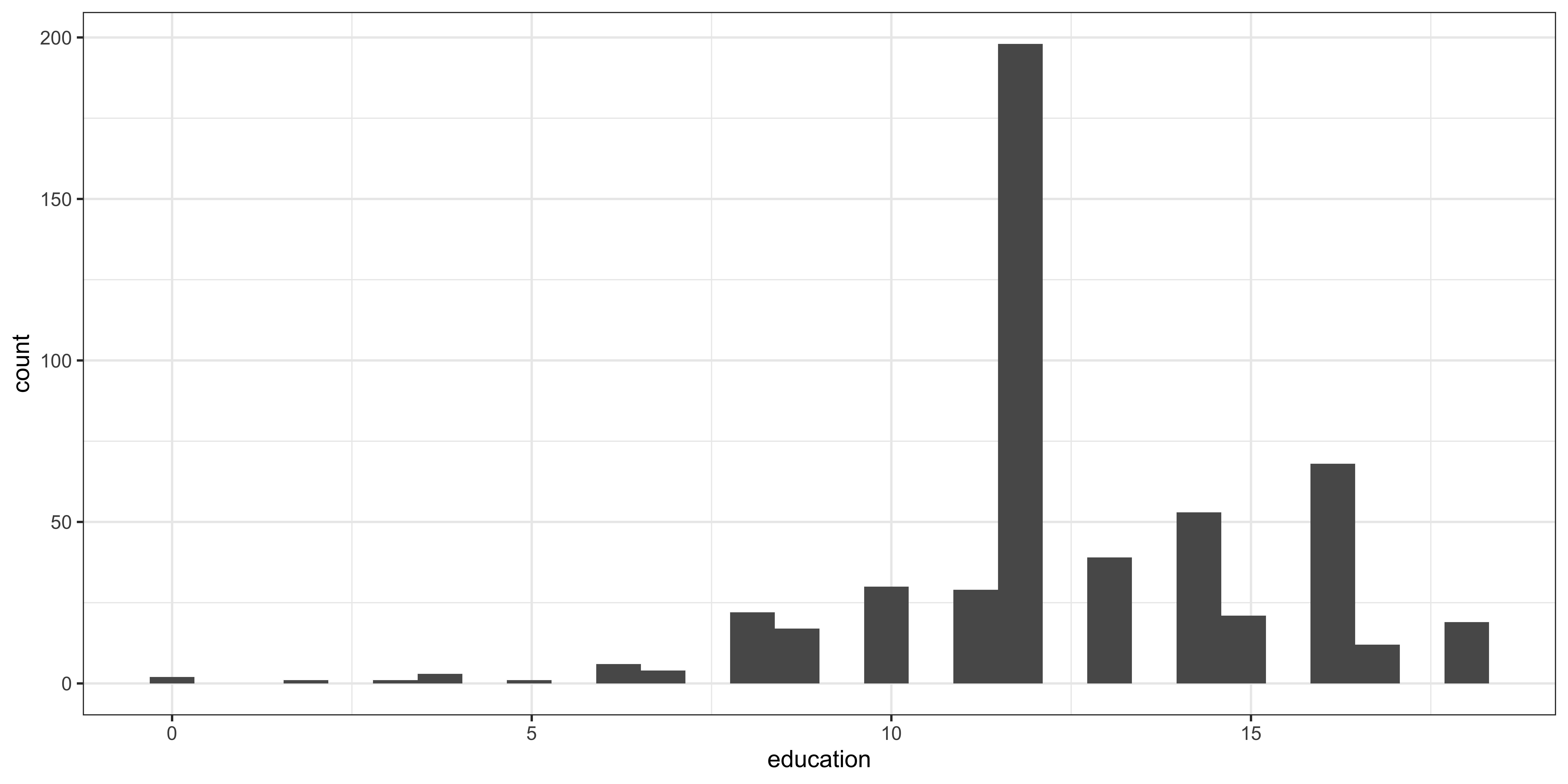
The code creates one thousand education values from the sample minimum to maximum and evaluates that expression at each value. In the left panel, the horizontal axis is education in years and the vertical axis is the marginal impact of experience, measured as dollars of hourly wage per additional year of experience. The horizontal reference line marks zero. The fitted effect begins negative at low education, increases linearly because the interaction coefficient is positive, and crosses zero at roughly zero point one eight eight divided by zero point zero two zero, about nine point two years of education. Above that value, the fitted experience slope is positive.

The right panel is a histogram of education. Its horizontal axis is again years of education and its vertical axis is the count of sample observations in each bin. Read the two panels together. The effect curve tells you what the model implies at each education value; the histogram tells you how much data support those evaluations. An effect near an education level with very few observations depends heavily on functional-form extrapolation.

The plot shows point estimates only. It does not include standard errors or a confidence band, so crossing the zero line does not by itself identify where the effect becomes statistically significant. For that we need the variance of the combination beta experience plus education times beta interaction. The next tabs construct a test at a particular education level.

Estimated Model

wage = 6.121 - 2.418 \times female - 0.188 \times exper + 0.020 \times educ \times exper


Marginal impact of experience

\frac{\partial wage}{\partial exper} = - 0.188 + 0.020 \times educ

Marginal impact of exper:
Histogram of education:
Transcript

This slide applies the quadratic-section logic to an interaction. Because the marginal impact of experience is negative zero point one eight eight plus zero point zero two zero times education, it varies with schooling. Substituting ten years gives about zero point zero one two dollars per hour for an additional year of experience using the rounded coefficients on screen. Substituting fifteen gives about zero point one one two dollars. These calculations are fitted marginal effects, not significance tests.

The research question below selects education equal to ten and asks whether the experience effect is positive or negative and statistically different from zero. In population notation, the null is beta experience plus ten times beta experience-education equals zero. The alternative says that combination is not zero. The interaction coefficient’s label stands for the coefficient on experience times education.

This is one linear restriction involving two population coefficients. A t-test of the combination is appropriate, or an equivalent one-restriction F-type test. Its numerator is beta hat experience plus ten beta hat interaction. Its variance is variance of beta hat experience, plus one hundred times variance of beta hat interaction, plus twenty times their covariance. Testing beta experience alone would ask about the experience slope at zero education. Testing the interaction alone would ask whether the experience slope changes with education. Neither is the question posed here.

The same framework can test fifteen years by replacing ten with fifteen. Because the estimated effect is larger there, the test may differ, but significance also depends on the combination’s standard error and the data available at that education level. The next tab asks R for the ten-year restriction.

Just like the case of the quadratic specification of education, marginal impact of experience is not constant

We can test if the marginal impact of experience is statistically significant for a given level of education

  • When educ=10, \frac{\partial wage}{\partial exper} = - 0.188 + 0.020 \times 10=0.012
  • When educ=15, \frac{\partial wage}{\partial exper} = - 0.188 + 0.020 \times 15=0.112

Question

Does an additional year of experience have a statistically significant impact (positive or negative) if your current education level is 10


Hypothesis

  • H_0: \beta_{exper} + \beta_{exper\_educ} \times 10=0

  • H_1: \beta_{exper} + \beta_{exper\_educ} \times 10\ne 0

Transcript

The code passes reg_int and one restriction string to car colon colon linearHypothesis. The string says the experience coefficient plus ten times the coefficient named I of experience times education equals zero. That is exactly the null from the previous tab at education equal to ten. Coefficient names inside the string must match the fitted model’s labels, including the capital I and the product term. If parsing fails, inspect names of coef reg_int and copy the stored label.

Using the unrounded estimates, the marginal effect at ten is about negative zero point one eight seven six plus ten times zero point zero two zero three seven, or positive zero point zero one six one dollars per hour. The test output gives a p-value of about zero point one one seven. At the five percent level, we therefore fail to reject the null that the experience effect is zero for a worker with ten years of education. The point estimate is positive, but it is not estimated precisely enough to distinguish from zero at that conventional level.

Do not turn “fail to reject” into proof of no effect. It means the sample and model do not provide sufficiently strong evidence against zero for this particular linear combination. It also does not settle the effect at fifteen years, where the combination and its standard error are different. The broader lesson is that whenever an interaction makes a marginal effect conditional on another variable, report both the conditioning value and the appropriate uncertainty for the full combination.

Including qualitative information


Including qualitative information

Transcript

So far our explanatory variables have naturally been numerical, such as education and experience. Many economically relevant characteristics are qualitative categories rather than measured amounts. The examples on screen include sex, marital status, and highest degree. Other examples would be region, crop type, treatment status, or occupation.

A regression still needs numerical columns, so we represent categories with indicator variables. For a binary characteristic such as married versus single, one zero-one variable contains all the information: code one for the category named by the variable and zero for the other category. Its coefficient compares those two groups, conditional on the other regressors.

For a characteristic with more than two states, such as high school, college, master’s, or doctoral degree, we need several indicators. With an intercept and c categories, include c minus one indicators. The omitted category becomes the baseline, and each included indicator coefficient measures a difference relative to it. Including all c indicators with an intercept creates exact redundancy because the indicators sum to one.

Coding does not create causality. A coefficient on a category describes a conditional mean difference after controlling for included variables, subject to the model assumptions. It should not automatically be labeled the effect of belonging to that category. We begin with binary variables, derive the comparison algebraically, and then extend the same idea to multiple categories and group-specific slopes.

Issue

How do we include qualitative information as an independent variable?


Examples

  • male or female (binary)

  • married or single (binary)

  • high-school, college, masters, or Ph.D (more than two states)

Transcript

The callout defines a dummy variable, also called an indicator or binary variable. It takes exactly two numerical values. One marks the category named by the variable and zero marks the other state. For example, in this dataset female equals one for women and zero for men; married equals one for married respondents and zero otherwise. The choice of which state receives one determines the sign and wording of the comparison, not the model’s fitted values.

The code beneath the definition uses dplyr colon colon select to keep six columns from wage1: wage, education, experience, female, and married, along with the listed variables, then pipes the result to head. Head displays the first six rows by default. Look across a row to see that continuous variables retain their measured values while female and married appear as zeros and ones. The pipe passes the selected table into head, making this a quick inspection rather than a transformation saved back to the data.

Why is zero-one coding convenient? In a regression, multiplying a coefficient by zero removes that category shift, while multiplying by one adds it. The conditional mean for the group coded one is therefore the baseline conditional mean plus the dummy coefficient. Subtracting the group-zero mean leaves exactly that coefficient. The next tab carries out this substitution for female and shows how “holding education fixed” enters the interpretation.

Dummy variable

  • Relevant information in binary variables can be captured by a zero-one variable that takes the value of 1 for one state and 0 for the other state

  • We use “dummy variable” to refer to a binary (zero-one) variable


Example

Transcript

The model is wage equals beta zero plus sigma f times female plus beta two times education plus u. Under the zero conditional mean assumption, the conditional expectation drops u. To interpret sigma f, evaluate the equation for each value of the dummy while keeping education at the same value.

For female equal to one, the conditional expected wage is beta zero plus sigma f plus beta two education. For female equal to zero, the sigma term disappears and expected wage is beta zero plus beta two education. Because zero identifies men in this coding, men are the baseline group. Subtract the second expression from the first. Beta zero and beta two education cancel, leaving sigma f. That is the equation displayed in the middle of the slide.

Verbally, sigma f is the expected hourly-wage difference between women and men who have the same education in this model. If sigma f is negative, women have the lower fitted conditional mean by its absolute value; if positive, they have the higher one. The comparison is conditional because education is held fixed. It is not the raw difference between average female and male wages, which could also reflect different education distributions.

Notice another restriction. The education coefficient beta two is identical for both groups, so this model permits different intercepts but forces parallel wage-education lines. Also avoid automatically interpreting sigma f as discrimination or a causal effect. Unobserved experience, occupation, hours, and other wage determinants remain in u and may differ by group. The next tab estimates this conditional mean difference, and the visualization after it makes the parallel-line restriction visible.

Model

wage = \beta_0 +\sigma_f female +\beta_2 educ + u


Interpretation

  • female: E[wage|female=1,educ] = \beta_0 + \sigma_f +\beta_2 educ

  • male: E[wage|female=0,educ] = \beta_0 + \beta_2 educ


This means that

\sigma_f = E[wage|female=1,educ]-E[wage|female=0,educ]

Verbally,

  • \sigma_f is the difference in the expected wage conditional on education between female and male

  • \sigma_f measures how much more (less) female workers make compared to male workers ( baseline ) if they were to have the same education level

Transcript

The code estimates the dummy-variable model with fixest colon colon feols. Wage is the dependent variable, and female plus education are the regressors. The data argument uses wage1. The result is stored as reg_df and then printed. Because no vcov option appears, the output uses fixest’s default IID standard errors.

The fitted female coefficient is about negative two point two seven three. Since female equals one for women and zero for men, read it as follows: among observations with the same education, the fitted hourly wage for women is about two dollars and twenty-seven cents lower than for men, on average. The inline R expression below the output pulls that exact coefficient from reg_df by its name, so the prose stays synchronized with the estimate rather than hardcoding a number.

The education coefficient is about zero point five zero six dollars per hour per additional year, and the intercept is about zero point six two three. Those terms define the baseline male line. Adding negative two point two seven three shifts that entire line downward for women. Because there is no female-times-education interaction, both groups share the same education slope.

Use conditional-association language. This regression controls only for education. It does not isolate discrimination, and it does not establish what the same person would earn under a different sex classification. Experience, occupation, tenure, work patterns, and many other factors are omitted and may be correlated with female. The coefficient is still a useful demonstration of dummy-variable interpretation, but the research design determines whether it has a causal meaning.

R implementation


Interpretation

Female workers make -2.2733619 ($/hour) less than male workers on average even though they have the same education level.

Transcript

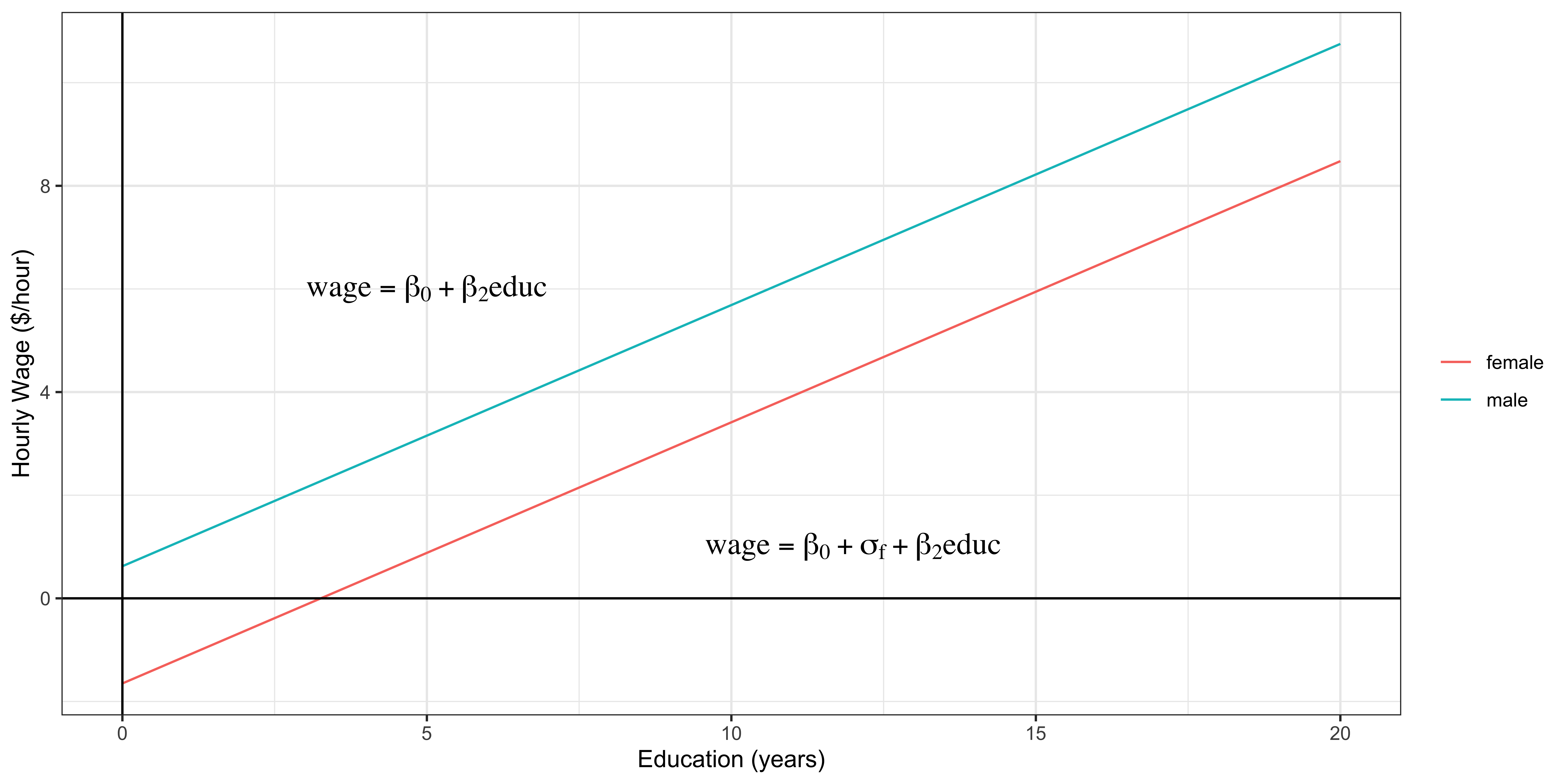
This figure draws the two fitted regression lines implied by the dummy-variable model. The horizontal axis is education in years and the vertical axis is hourly wage in dollars. The legend distinguishes female and male. The male line is beta zero plus beta two times education because female equals zero. The female line is beta zero plus sigma f plus beta two times education because female equals one. The text labels on the plot write those two equations next to their lines.

Both lines have slope beta two, so they are parallel. Their vertical separation at every education value is sigma f. In this fitted model sigma f is negative, so the female line lies below the male line by about two point two seven dollars per hour everywhere. The code constructs education values from zero to twenty, evaluates each equation, combines the two data tables, and maps line color to group. The vertical and horizontal reference lines mark zero on the axes; they are coordinate guides, not estimated effects.

The picture reveals the restriction more clearly than the table. Adding a dummy by itself allows the intercept to differ across groups but does not allow the education slope to differ. If the lines actually converge, diverge, or cross, this model cannot represent that behavior. You would need a female-times-education interaction, which adds gamma to the female slope. Also notice that the plotted lines extend to zero education, even if that region has limited sample support. Interpret fitted differences primarily where the data exist. We first examine how changing the dummy coding affects the same parallel-line model.
Transcript

Now recode the same two categories with male equal to one and female equal to zero. The model is wage equals beta zero plus sigma m times male plus beta two education plus u. The algebra is identical, but the baseline changes.

For male equal to one, expected wage is beta zero plus sigma m plus beta two education. For male equal to zero, which now means female, expected wage is beta zero plus beta two education. Subtracting the female expression from the male expression leaves sigma m. Thus sigma m is the conditional expected wage difference, male minus female, at the same education level.

Compare this with the earlier female coding. Sigma f represented female minus male, so sigma m must be the negative of sigma f. The new intercept is the old intercept plus sigma f because the baseline line has switched from men to women. The education slope and every fitted wage remain unchanged. Coding changes the parameter labels and signs, not the substantive model.

The callout gives the general rule: whichever category receives zero is the baseline. State that baseline whenever you report a categorical coefficient. There is no universally correct choice. Pick a reference group that makes the comparisons meaningful or conventional for the application. The next tab verifies the sign and intercept changes in R.

Model

wage = \beta_0 +\sigma_m male +\beta_2 educ + u


Interpretation

  • male: E[wage|male = 1,educ] = \beta_0 + \sigma_m +\beta_2 educ

  • female: E[wage|male = 0,educ] = \beta_0 + \beta_2 educ


This means that

\sigma_m = E[wage|male=1,educ]-E[wage|male=0,educ]

Verbally,

  • \sigma_m is the difference in the expected wage conditional on education between male and female

  • \sigma_m measures how much more (less) male workers make compared to female workers (baseline) if they were to have the same education level

Important

Whichever status that is given the value of 0 becomes the baseline

Transcript

The first code line creates male as one minus female. Because female is zero or one, this reverses the coding exactly: a female value of zero becomes male equal to one, and a female value of one becomes male equal to zero. Dplyr mutate returns the updated wage1 data with the new column.

The feols call then regresses wage on male and education. Wage1 is supplied through the data argument, and the fitted object is again named reg_df. The output shows a male coefficient of about positive two point two seven three, exactly the opposite sign of the earlier female coefficient. The intercept is about negative one point six five one rather than positive zero point six two three because it now describes the fitted female wage at zero education. The education coefficient remains about zero point five zero six.

The inline interpretation extracts the male coefficient by name. With women as the zero-coded baseline, men have a fitted hourly wage about two dollars and twenty-seven cents higher at the same education level. This says the same thing as women having a fitted wage two dollars and twenty-seven cents lower than men.

You can verify prediction invariance algebraically. For a man, the new equation adds the male coefficient to the new intercept, recovering the old male intercept. For a woman, it leaves the new intercept, which equals the old intercept plus the old female shift. Nothing about residuals, fitted values, R squared, or substantive conclusions changes. Only the reference category and coefficient parameterization change.

Regression results


Interpretation

Male workers make NA ($/hour) more than female workers on average even though they have the same education level.

Transcript

Before opening the answer, write the identity connecting these columns. For every observation, male plus female equals one. A regression intercept is itself a column of ones. Therefore the intercept column equals male plus female exactly.

If the model includes an intercept, male, and female, one regressor column is a perfect linear combination of the others. This is perfect multicollinearity. The design matrix does not have full column rank, so the normal equations cannot identify a unique coefficient on all three columns. Many coefficient triples produce the same fitted values because you can shift the intercept and offset both dummy coefficients without changing a prediction.

The answer panel lists the consequences. Male and female contain redundant information once the intercept is present. To estimate the model, drop either male or female and interpret the remaining indicator relative to the omitted group. This is the dummy-variable trap. More generally, with c mutually exclusive and exhaustive categories and an intercept, include c minus one category indicators.

An alternative is to omit the intercept and include all category indicators. Then each category coefficient can represent its own intercept, but the interpretation and other formula terms must be handled carefully. The standard approach in this course is to keep the intercept and omit one baseline category. The next tab lets you see how software handles the redundant specification.

What do you think will happen if we include both male and female dummy variables?


Answer
  • They contain redundant information

  • Indeed, including both of them along with the intercept would cause perfect collinearity problem

  • So, you need to drop either one of them

Transcript

The equation above the code states the exact dependence: intercept equals male plus female. The feols formula nevertheless requests wage on male, female, and education. Because those columns are perfectly collinear, all requested coefficients cannot be estimated uniquely.

When this cell runs, fixest detects the collinearity and removes female. It estimates the remaining model with an intercept, male, and education, then prints a message that one variable was removed because of collinearity. The reported coefficients match the male-baseline-choice regression from the previous tab because that is the estimable parameterization fixest retained.

The automatic removal prevents a matrix-inversion failure, but it should not be treated as permission to ignore the problem. The software’s choice of which variable to drop may depend on term order and implementation. If you overlook the message, you may interpret a baseline you did not intend or believe that a requested coefficient was estimated when it was not. Always inspect the coefficient table, removal notes, and stored collinearity information.

The proper remedy is to specify the reference category deliberately. Include either female or male, not both, when retaining the intercept. For a multi-category variable, use c minus one indicators or a factor-aware helper that explicitly names the reference. This preserves full rank and makes the comparison clear in the code and writeup. The next section returns to female coding and adds an interaction so the groups can differ in slope as well as intercept.

In the model, intercept = male + female, which causes perfect collinearity.

Here is what happens if you include both:


One of the variables that cause perfect collinearity is automatically dropped.

Interactions with a dummy variable

Interactions with a dummy variable

Transcript

The first bullet recalls the restriction in the dummy-only model: women and men could have different fitted wage levels, but education had exactly the same slope for both. The question here is whether we can allow the marginal association between education and wage to differ by group. We can, by interacting the female indicator with education while retaining both main effects.

Read the flexible model term by term. Beta zero is the male intercept because male is the female-equals-zero baseline. Sigma f times female allows the female intercept to differ. Beta two times education is the male education slope. Gamma times female times education allows that slope to change for women.

Substitute female equal to zero. Both terms containing female disappear, leaving expected wage for men equal to beta zero plus beta two education. Substitute female equal to one. The intercept becomes beta zero plus sigma f, and the two education terms combine into beta two plus gamma times education. Thus the model gives each group its own intercept and slope.

Gamma is the female education slope minus the male education slope. If gamma is positive, the fitted return to another year of schooling is larger for women; if negative, it is smaller. Sigma f now has a narrower interpretation than in the parallel-lines model: it is the female-minus-male wage difference at education equal to zero. At education level e, the fitted group gap is sigma f plus gamma times e, so it can widen, narrow, or cross zero.

Because zero education may not be a useful reference, you could center education at a meaningful value before interacting. Then sigma f would describe the group gap at that reference level while fitted values remain unchanged. The next tab estimates this full hierarchical specification.

  • In the previous example, the impact of education on wage was modeled to be exactly the same

  • Can we build a more flexible model that allows us to estimate the differential impacts of education on wage between male and female?

A more flexible model

wage = \beta_0 + \sigma_f female +\beta_2 educ + \gamma female\times educ + u

  • female: E[wage|female=1,educ] = \beta_0 + \sigma_f +(\beta_2+\gamma) educ
  • male: E[wage|female=0,educ] = \beta_0 + \beta_2 educ


Interpretation

For female, education is more effective by \gamma than it is for male.

Transcript

The feols formula includes female, education, and I of female times education. Including all three respects the hierarchy rule: the two main effects remain alongside their product. Capital I tells the formula parser to multiply the two columns literally. The data argument uses wage1, and the surrounding parentheses cause the fitted model, stored as reg_di, to print immediately.

The output gives an intercept of about zero point two zero zero, a female coefficient of about negative one point one nine nine, an education coefficient of about zero point five three nine, and an interaction coefficient of about negative zero point zero eight six. No vcov argument is supplied, so these are paired with the default IID standard errors.

Interpret the slopes by substituting dummy values. For men, female equals zero, so the marginal effect of education is beta education, about fifty-four cents of hourly wage per additional year. For women, female equals one, so the marginal effect is beta education plus beta interaction, about zero point five three nine minus zero point zero eight six, or roughly forty-five cents. The interaction estimate is the difference between those slopes: the fitted education slope is about eight point six cents lower for women.

The female main-effect coefficient is not an overall group gap. In this interacted model it is the fitted female-minus-male difference at zero years of education. At education e, the gap is negative one point one nine nine minus zero point zero eight six times e. Also check uncertainty. The interaction t-statistic is about negative zero point eight three with p about zero point four zero seven, so this sample does not provide evidence that the slopes differ from zero at conventional levels. The next tab visualizes the point estimates and makes the changing group gap visible.

Transcript

The statement above the graph interprets gamma, the coefficient on female times education. Its estimate is negative zero point zero eight six, so the fitted marginal benefit of one more year of education is about eight point six cents per hour lower for women than for men. This is a difference in slopes, not the wage gap at a particular schooling level.

The graph has education in years on the horizontal axis and hourly wage in dollars on the vertical axis. The male line uses beta zero plus beta two education. The female line uses beta zero plus sigma f plus beta two plus gamma times education. The labels printed beside the lines show those equations, and the color legend identifies the groups. The vertical and horizontal lines mark zero on the axes.

Unlike the earlier dummy-only picture, these lines are not parallel. The male slope is about zero point five three nine, while the female slope is about zero point four five three. Because gamma is negative, the female line rises more slowly. Sigma f is also negative, so the female line starts below the male line at zero education and the fitted gap becomes more negative as education rises. At any education e, that gap is sigma f plus gamma e.

The figure displays fitted point estimates and does not show confidence bands. The interaction coefficient’s p-value is about zero point four zero seven, so we cannot statistically distinguish the estimated slope difference from zero at conventional levels. That uncertainty should accompany the point interpretation. Since gamma is one coefficient in this parameterization, its printed t-test directly addresses equality of the two education slopes. Testing whether the groups have identical regression lines altogether would require jointly testing both sigma f and gamma.

The marginal benefit of education is 0.086 ($/hour) less for females workers than for male workers on average.
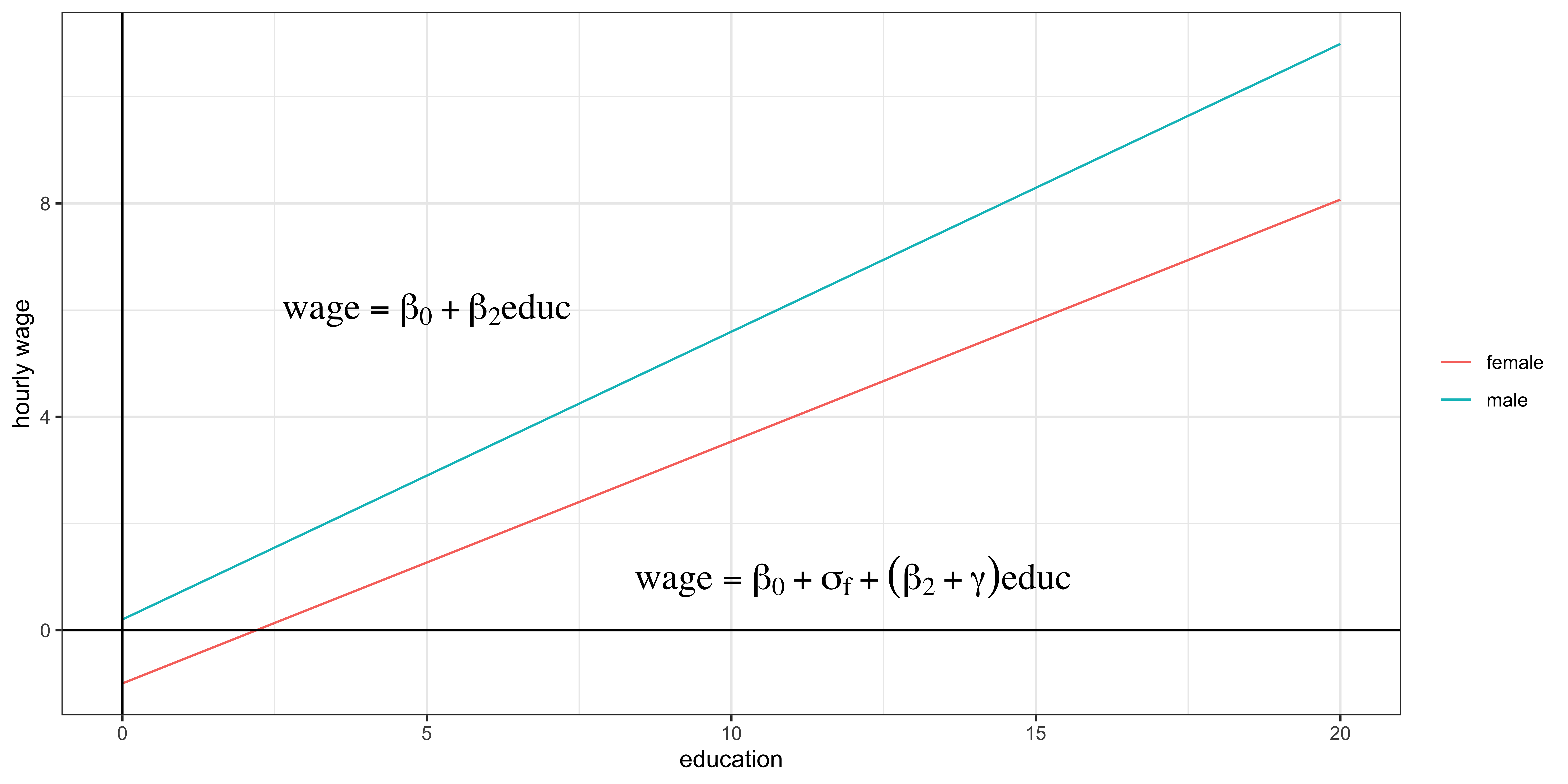
Categorical variable: more than two states

Transcript

Now move from a binary variable to a categorical variable with three states. The example degree variable records whether the highest degree is college, master’s, or doctoral. A single zero-one variable cannot distinguish all three states, so we define one indicator for each category: college equals one only for college graduates, master equals one only for master’s graduates, and doctor equals one only for Ph.D. graduates.

For every observation exactly one of those indicators equals one, so college plus master plus doctor equals one. With an intercept, including all three would recreate perfect collinearity because their sum equals the intercept column. The rule is therefore to include the number of categories minus one. With three states, include two indicators and omit one.

The omitted indicator is not discarded substantively. Its category becomes the baseline represented by the intercept and the other common regression terms. Each included dummy coefficient compares its category with that baseline, holding the other regressors fixed. If college is omitted, the master coefficient is master minus college, and the doctor coefficient is doctor minus college.

You may choose a different baseline to answer a different comparison directly. Omitting master, for example, would make the doctor coefficient compare Ph.D. with master’s. Regardless of coding, the model spans the same category-specific conditional means and produces the same fitted values. Modern R functions can create these indicators from one categorical column automatically, which we show later. The next tab derives the three group-specific expectations when college is the omitted category.

  • Consider a variable called degree which has three status values: college, master, and doctor.

  • Unlike a binary variable, there are three status values.

  • How do we include a categorical variable like this in a model?

What do we do about this?

You can create three dummy variables like below:

  • college: 1 if the highest degree is college, 0 otherwise
  • master: 1 if the highest degree is Master’s, 0 otherwise
  • doctor: 1 if the highest degree is Ph.D., 0 otherwise

You then include two (the number of status values - 1) of the three dummy variables:

Transcript

The model includes master and doctor indicators but omits college, so college is the baseline. It also includes education as a continuous regressor. Under the conditional mean assumption, evaluate the equation for each feasible indicator pattern while holding education fixed.

For a college graduate, master and doctor both equal zero. Expected wage is beta zero plus beta one education. For a master’s graduate, master equals one and doctor equals zero, so expected wage is beta zero plus sigma m plus beta one education. For a Ph.D. graduate, master equals zero and doctor equals one, giving beta zero plus sigma d plus beta one education. The impossible combination master equals one and doctor equals one should not occur if highest degree is coded correctly.

Subtract the college expression from the master’s expression and only sigma m remains. It is the fitted wage difference between master’s and college graduates at the same education level. Sigma d similarly compares Ph.D. with college. Neither coefficient directly compares master’s with Ph.D. That difference is sigma d minus sigma m, and testing equality of those two categories requires the restriction sigma d minus sigma m equals zero.

The common beta one term means this model forces the same education slope across all degree categories. If the return to an additional year differs by degree, interact the category indicators with education. Also think carefully about including both highest degree and years of education: they are related but not identical, and the coefficient interpretation is conditional on the other. Finally, use “conditional difference” unless a research design supports causal language. The red phrases emphasize relativity: every dummy coefficient must be interpreted against the omitted college baseline.

Model

wage = \beta_0 + \sigma_m master +\sigma_d doctor + \beta_1 educ + u

  • college: E[wage|master=0, doctor = 0, educ] = \beta_0 + \beta_1 educ
  • master: E[wage|master=1, doctor = 0, educ] = \beta_0 + \sigma_m + \beta_1 educ
  • doctor: E[wage|master=0, doctor = 1, educ] = \beta_0 + \sigma_d + \beta_1 educ


Interpretation

\sigma_m: the impact of having a MS degree relative to having a college degree

\sigma_d: the impact of having a Ph.D. degree relative to having a college degree


Important

The omitted category (here, college) becomes the baseline.

Structural differences across groups

Transcript

Structural difference means that the conditional relationship itself can differ across groups, not merely that one group has a constant level shift. The example models cumulative college GPA separately for male and female athletes. Cumgpa is cumulative grade point average, sat is SAT score, hsperc is high-school rank percentile, and tothrs is total completed college credit hours.

Look at the two equations. The male model uses alpha zero through alpha three. The female model uses beta zero through beta three. Allowing every coefficient to differ means the groups may have different intercepts, different SAT slopes, different high-school-rank slopes, and different credit-hour slopes. For hsperc, remember that a larger percentile value in this dataset corresponds to a different rank position according to its coding; the coefficient interpretation must follow the variable definition.

If the true group relationships differ this broadly, a single pooled equation with common slopes imposes false equality restrictions. Its common coefficients can become a weighted compromise between two functions and may describe neither group well. On the other hand, estimating completely separate regressions without testing can waste precision if the functions are actually the same.

The econometric task is therefore to formulate and test equality of the group-specific parameters. “Fundamentally different” does not mean every estimate must visibly differ or every separate t-test must be significant. It means we consider a joint hypothesis about the whole coefficient vector. The next tab shows how one interacted regression can contain both group equations and turn structural equality into a set of testable restrictions.

Structural difference refers to the fundamental differences in the model of a phenomenon in the population:


Example

Male: cumgpa = \alpha_0 + \alpha_1 sat + \alpha_2 hsperc + \alpha_3 tothrs + u

Female: cumgpa = \beta_0 + \beta_1 sat + \beta_2 hsperc + \beta_3 tothrs + u

  • cumgpa: college grade points averages for male and female college athletes

  • sat: SAT score

  • hsperc: high school rank percentile

  • tothrs: total hours of college courses


In this example,

cumgpa are determined in a fundamentally different manner between female and male students.

You do not want to run a single regression that fits a single model for both female and male students.

Transcript

If you suspect structural differences, do not simply assume separate models. Estimate a flexible unrestricted specification and test whether the extra group-difference terms are needed. The displayed equation does this inside one regression by using female as the group indicator and interacting it with every explanatory variable.

Read the equation line by line. Beta zero is the male intercept, and sigma zero times female permits the female intercept to differ. Beta one sat is the male SAT slope, while sigma one times sat times female changes that slope for women. The same pairing appears for hsperc and tothrs. All main effects are retained alongside their interactions, which satisfies the hierarchy rule.

Set female equal to zero and every sigma term disappears. You recover the male equation with beta zero, beta one, beta two, and beta three. Set female equal to one and collect terms. The female intercept becomes beta zero plus sigma zero; the SAT slope becomes beta one plus sigma one; the hsperc slope becomes beta two plus sigma two; and the credit-hours slope becomes beta three plus sigma three.

This parameterization is useful because each sigma is a female-minus-male difference in one structural coefficient. If all sigmas equal zero, the same regression function applies to both groups. If at least one differs, the functions are structurally different under this specification. Estimating everything in one model also provides the full covariance matrix needed for a joint test. The next tab writes the group equations explicitly and identifies the appropriate null.

If you suspect that the underlying process of how the dependent variable is determined vary across groups, then you should test that hypothesis!


To do so,

You estimate the model that allows to estimate separate models across groups within a single regression analysis.


A more flexible model

cumgpa = \beta_0 + \sigma_0 female + \beta_1 sat + \sigma_1 (sat \times female) \;\; + \beta_2 hsperc + \sigma_2 (hsperc \times female) \qquad + \beta_3 tothrs + \sigma_3 (tothrs \times female) + u

Transcript

The first two lines are the group-specific conditional means obtained from the flexible model. For men, female equals zero, so expected cumulative GPA is beta zero plus beta one SAT plus beta two high-school percentile plus beta three total hours. For women, female equals one, so each corresponding coefficient is beta plus sigma. This confirms that one pooled interacted equation reproduces two fully separate linear functions.

The bullets summarize the parameter roles. The betas are the baseline male coefficients and also the common components of the female coefficients. Each sigma measures a female-minus-male difference: sigma zero for the intercept, sigma one for the SAT slope, sigma two for the hsperc slope, and sigma three for the tothrs slope.

The verbal null says the male and female GPA models are not structurally different. Mathematically, that means sigma zero, sigma one, sigma two, and sigma three all equal zero simultaneously. Count the restrictions: there are four equations. That makes this a joint test, conventionally presented as an F-test in a finite-sample linear model, rather than a t-test of one coefficient.

Four separate t-tests would not answer the same single joint question. They ignore covariance among estimates and create a multiple-testing issue. It is possible for no individual coefficient to cross the five percent threshold while the four coefficients are jointly far from zero. Open the answer and you see “F-test.” In software using large-sample covariance methods, the same joint Wald idea may be reported with a chi-squared statistic. The important distinction is one restriction versus several restrictions, not merely the label printed by the function.

Male: E[cumgpa] = \beta_0 + \beta_1 sat + \beta_2 hsperc + \beta_3 tothrs Female: E[cumgpa] = (\beta_0 +\sigma_0) + (\beta_1+\sigma_1) sat + (\beta_2+\sigma_2) hsperc + (\beta_3+\sigma_3) tothrs


Interpretation

  • \betas are commonly shared by female and male students
  • \sigmas capture the differences between female and male students

Null Hypothesis

  • (verbally) The model of GPA for male and female students are not structurally different.
  • (mathematically) H_0: \;\; \sigma_0=0,\;\; \sigma_1=0, \;\; \sigma_2=0, \;\; \text{and} \;\; \sigma_3=0

Question

What test do we do? t-test or F-test?


Answer F-test.
Transcript

This code prepares the GPA data and estimates the unrestricted group-specific model. Data with the name gpa3 is loaded from the wooldridge package. The pipeline starts from gpa3 and uses dplyr filter with not is dot n a of ctothrs, retaining only observations for which ctothrs is observed. That sample restriction matters: the fitted model describes the retained observations, not every row in the original data. Record and justify such filtering in an empirical writeup.

Dplyr mutate then creates three products explicitly. Female_sat is female times sat, female_hsperc is female times hsperc, and female_tothrs is female times tothrs. The colon-equals syntax supplies the new column names. Storing the resulting table as gpa lets the regression reuse those terms.

Fixest feols estimates cumgpa on seven regressors. Female allows an intercept difference. Sat, hsperc, and tothrs are the baseline male slopes. Each female product allows the corresponding female slope to differ. The formula is split across lines only for readability. The data argument points to gpa, and the fitted unrestricted model is stored as reg_full for later output and testing. No vcov argument is specified, so fixest uses IID standard errors.

The cell does not print reg_full, so its main purpose is preparation. Autorun ensures later cells can use the object. A more compact formula could use interactions directly, but explicit columns make the coefficient names easy to pass to linearHypothesis. The next tab prints the estimates and asks why their separate p-values are not enough.

Run the unrestricted model with all the interaction terms:

Transcript

Summary of reg_full prints the unrestricted coefficient table and fit information. There are 366 observations in the filtered sample. The baseline male coefficients are the intercept and the coefficients on sat, hsperc, and tothrs. The female coefficient changes the intercept, while female_sat, female_hsperc, and female_tothrs change the three slopes for women.

Focus on the four female-related rows. The female intercept difference has p about zero point three nine. Female_sat has p about zero point zero five two, close to but still above five percent. Female_hsperc has p about zero point eight six, and female_tothrs has p about zero point nine four. Thus none is individually significant at the five percent level.

The tempting conclusion is that men and women have the same regression function. That does not follow. Each t-test asks whether one difference coefficient is zero while leaving the others unrestricted. Structural equality asks whether all four are zero at once. The coefficient estimates are correlated because each interaction is built from the same group indicator and related covariates. A collection of moderately unusual estimates can provide strong joint evidence even when no single standardized estimate passes its individual cutoff.

This is not a request to reinterpret near-significant p-values. It is a request to test the actual multi-parameter hypothesis. We need a joint Wald or F-type test using the covariance matrix of all four estimates. The next tab performs it in one call.

Regression results


What do you see?

  • None of the variables that involve female are statistically significant at the 5% level individually.

  • Does this mean that male and female students have the same regression function?

  • No, we are testing the joint significance of the coefficients. We need to do an F-test!

Transcript

The linearHypothesis call supplies reg_full as the fitted unrestricted model and a character vector containing four restrictions. The c function combines the strings. They set the female intercept difference, female_hsperc, female_sat, and female_tothrs equal to zero. The order of the restrictions does not matter, but each stored coefficient name must match the model output.

Together these restrictions state that the female equation has the same intercept and all three of the same slopes as the male equation. The function uses the model’s coefficient covariance matrix to construct one joint statistic. With the current fixest and car methods, the output is labeled chi-squared: about thirty-two point seven on four restrictions, with p about one point four times ten to the minus six. In the classical finite-sample presentation, the corresponding joint test is discussed as an F-test. Both formulations address the same structural-equality null.

The p-value is far below one percent, so we reject the joint null. The data provide strong evidence that at least one of the four group-difference parameters is nonzero under this model. That does not tell us that all four differ, nor does it identify which difference is causal. It says the complete male and female regression functions should not be treated as identical.

Compare this conclusion with the previous tab: no female-related term was individually significant at five percent, yet the set is strongly significant jointly. That contrast is exactly why the test must match the hypothesis. Whenever your verbal claim involves several coefficients at once, write all restrictions and use a joint test rather than scanning individual stars.

R coding tips: categorical variables and interaction terms

Transcript

This practical section shows how categorical data are commonly represented in R. The original big9salary data contain separate zero-one columns for universities. Real analysis is usually easier when one column stores the category label, so the code reconstructs a university column before using fixest’s factor helpers.

The data call loads big9salary from wooldridge. As_tibble converts it to a tibble for readable dplyr work. Mutate creates university with case_when. Each condition checks whether one university indicator equals one; the value to the right of the tilde is the label assigned when that condition is true. For example, osu equal to one becomes “Ohio State U,” and msu equal to one becomes “Michigan State U.” Case_when evaluates conditions in order, so mutually exclusive indicators are expected.

There is an important data-preparation detail visible in the code: only eight named indicators are mapped and there is no final default condition. Any row for the original omitted university, where all eight displayed indicators equal zero, receives a missing university value. Later regressions using university will omit such rows. When reconstructing a categorical variable in your own data, explicitly map the reference category too, often with a final condition after verifying the indicator system.

Finally, relocate moves id, year, salary, pubindx, and university to the front of the table without dropping the remaining columns. The transformed object is stored as big9salary_c. The goal is a readable single category column that functions can expand into indicators consistently. The next tab inspects the beginning and end of this result before modeling it.

Transcript

This cell inspects the reshaped data from both ends. Head of big9salary_c prints the first six rows by default, and tail prints the last six. Because the two expressions are separate, the output shows two small tables one after the other.

Focus on the columns relocated to the front. Id identifies the faculty member, year gives the observation year, salary is the annual salary outcome, pubindx is the publication index, and university is the new text category. For rows matched by case_when, one university label now carries information that was previously scattered across several dummy columns. The original columns still remain later in the tibble because relocate changes order rather than selecting a subset.

This one-column representation is easier to inspect, filter, summarize, and pass to modeling functions. It also avoids hand-maintaining c minus one dummy columns every time categories change. However, inspect missing values as well as visible labels. Rows for a category not covered by the case_when mapping have university equal to missing, and a regression that uses university will drop them. Head and tail alone may not reveal every category or missingness pattern, so in real work also count university values, including missing values, before estimating.

Once the category column is verified, the next tab uses fixest’s i function to create the regression indicators and declare the baseline in the formula itself.

Take a look at the data,

Transcript

The formula uses fixest’s i function to handle university as a categorical regressor. Salary is the dependent variable. Pubindx and female enter as ordinary controls. I of university creates the needed category indicators, while ref equals “Indiana U” explicitly selects Indiana as the omitted baseline. The data argument uses big9salary_c. The fitted model is piped into broom tidy, which returns one row per coefficient with estimates, standard errors, test statistics, and p-values.

Each university coefficient is an intercept difference relative to Indiana, holding publication index and female fixed. A negative Michigan State coefficient means faculty at Michigan State have a lower fitted annual salary than otherwise comparable faculty at Indiana by the coefficient’s absolute dollar amount. It is not a comparison with the overall average or with every other university. To compare Michigan State with Michigan, for example, you would take the difference between those two indicator coefficients and compute its standard error.

The ref argument makes the baseline visible and reproducible. That is safer than manually creating dummies, accidentally including all categories with an intercept, or relying on an implicit alphabetical reference. The function automatically includes c minus one estimable indicators and adapts if verified categories change.

Read the output’s sample note too. Observations with missing salary, female, pubindx, or university are removed. Because the preparation code leaves the original all-zero category unmapped, university missingness contributes to that omission. Indicator automation solves formula coding, not data validation. Once the category column is correct, i of category variable is the concise approach to use.

You can use the i() function inside fixest::feols() like below:


ref = "Indiana U" sets the base category to "Indiana U".

So, for example, the highlighted line means that faculty members at Michigan State U make 9,118 USD less annually than those at Indiana U.


Key

You do not have to make a bunch of dummy variables like the original dataset. Just use i(category_variable).

Transcript

The research question now asks whether the association between publication index and salary varies by university. The formula retains female and pubindx as main effects. The first i term, i of university with Indiana as reference, allows university intercepts to differ. The second i term passes pubindx as the continuous variable and again sets Indiana as the reference; it creates university-by-pubindx interaction terms that allow slopes to differ.

Interpret the main pubindx coefficient first. It is the fitted salary change for a one-unit increase in publication index at the baseline Indiana University. Each interaction coefficient is an additional slope relative to Indiana. For Michigan State, the interaction estimate is about four hundred thirty-six dollars. Its fitted publication-index slope is therefore the Indiana slope plus four hundred thirty-six, not four hundred thirty-six alone. The slide’s final sentence correctly frames the interaction as a marginal-impact difference.

The ordinary university indicators are still needed. Without them, the specification would force all university lines to share an intercept at pubindx equal to zero while allowing only slopes to differ. Including both sets gives each nonbaseline university an intercept adjustment and a slope adjustment, the categorical analogue of interacting a dummy with education.

Broom tidy exposes all coefficients and their uncertainty. A t-test on one interaction compares that university’s slope with Indiana’s. A joint test setting every university-pubindx interaction to zero asks whether publication returns are the same across all represented institutions. That is the same structural-difference logic as the GPA example, now generated compactly with i rather than hand-built product columns. Be precise that the variable is named pubindx in the data and code.

You can use i() for creating interactions of a categorical variable and a continuous variable.

Suppose you are interested in understanding the impact of pubindx (continuous) by university (categorical), then


So, the marginal impact of pubindex is 436 greater for those at Michigan State U than those at Indiana U.

Other miscellaneous topics


Goodness of fit: R^2

Transcript

The callout makes a deliberately strong statement: a small R squared is often not a serious problem. To understand it, separate goodness of fit from identification. R squared is one minus the residual sum of squares divided by the total sum of squares when the usual intercept is present. It measures the fraction of sample variation in the dependent variable accounted for by the fitted values. A value near one means observations lie close to the fitted regression surface; a value near zero means much outcome variation remains in the residuals.

That statistic does not tell you whether a coefficient is unbiased, causal, or even economically sensible. A model can fit extremely well because it includes variables correlated with the outcome while still suffer severe endogeneity. Conversely, a randomized regressor can identify a causal effect cleanly even when many other determinants of the outcome remain unexplained and R squared is low.

Whether fit matters depends on the goal. For prediction, unexplained variation and out-of-sample performance are central, although in-sample R squared alone is still not enough. For estimating a particular causal or structural parameter, the crucial questions concern exogeneity, research design, correct specification of the relevant relationship, and valid uncertainty. Adding irrelevant or endogenous controls merely to raise R squared can make the analysis worse.

So “we could not care less” should be read in context. Do report fit honestly, and investigate coding errors or obvious misspecification. But do not treat R squared as a grade for a causal regression. The apple example on the next tabs shows a low R squared alongside a credible price-effect design.

Important

Small value of R^2 does not mean the end of the world (In fact, we could not care less about it.)

Transcript

The example regression has ecolabs, described in the bullets as the hypothetical pounds of eco-labeled apples a family would demand, on the left. Regprc is the price of regular apples, and ecoprc is the experimentally assigned price of eco-labeled apples. Beta one captures how demand changes with the regular-apple price, holding the eco price fixed. Beta two captures how demand changes with the eco-apple price, holding the regular price fixed.

The key design fact is in the first bullet: the researcher randomly set ecoprc when constructing the survey scenarios. Random assignment breaks systematic association between the assigned price and unobserved demand determinants, supporting the zero conditional mean condition for causal interpretation of that price coefficient. The slide also states the study’s narrow objective, understanding how eco-apple demand responds to the eco-apple price.

Family demand can still vary for many reasons not in this short equation: income, household size, preferences, environmental attitudes, and ordinary idiosyncratic choices. Those omitted determinants increase residual variation and lower R squared. They do not bias the randomized price coefficient merely because they are omitted, provided randomization makes them unrelated to assigned price in expectation.

That is the central distinction. R squared asks how much individual demand variation the model explains. Identification asks whether variation in ecoprc is exogenous enough to recover its causal effect. Randomization can answer the second question even when the first answer is “very little.” The next tab runs the regression and lets you compare a small fit statistic with precise price estimates.

Example

ecolabs = \beta_0 + \beta_1 regprc + \beta_2 ecoprc

  • ecolabs: the (hypothetical) pounds of ecologically friendly (eco-labeled) apples a family would demand
  • regprc: prices of regular apples
  • ecoprc: prices of the hypothetical eco-labeled apples


Key

  • The data was obtained via survey and ecoprc was set randomly (So, we know E[u|x] = 0) by the researcher.
  • The (only) objective of the study is to understand the impact of the price of eco-labeled apple on the demand for eco-labeled apples.
Transcript

The code loads apple from the wooldridge package, then estimates ecolbs on regprc and ecoprc with fixest feols. Notice that the dataset’s actual outcome name in code is ecolbs. The surrounding parentheses print the fitted model immediately. No vcov argument is shown, so the table uses IID standard errors.

The fitted intercept is about one point nine six five. The regular-apple price coefficient is positive three point zero two nine, consistent with regular and eco-labeled apples acting as substitutes in this survey: a higher regular price is associated with greater demand for eco apples. The eco-apple price coefficient is negative two point nine two six, so raising the eco price by one price unit reduces hypothetical eco-apple demand by about two point nine three pounds, holding regular price fixed. Both price coefficients have very small p-values in the displayed regression.

The ordinary R squared is about zero point zero three six, and the adjusted R squared shown by fixest is about zero point zero three three. Thus the two price variables explain only a few percent of the sample variation in stated demand. Open the answer: that low value is not a problem for the stated objective. The study seeks the causal response to assigned price, not a high-accuracy prediction of each family’s pounds demanded.

Randomizing the survey price provides credibility that a higher-demand family was not systematically assigned a different ecoprc. Adding variables solely to inflate R squared would not improve that randomization. Covariates might improve precision if chosen appropriately, but fit is not the identification argument. The answer is therefore no, while still leaving room to scrutinize survey realism, compliance with the hypothetical scenario, standard errors, and external validity.


Question

Note that R^2 is very small. Is this a problem?


Answer

No.

  • Their goal is not predicting the demand of eco-labeled apple. Understanding the causal impact of price on demand.
  • The goal is achieved via randomization of the price variables at the stage of designing the survey!

Scaling

Transcript

This section asks what changes when you rescale a variable used in a regression. Think of measuring education in months instead of years, income in thousands of dollars instead of dollars, or land in hectares instead of acres. The underlying observations and economic relationship have not changed; only the numerical unit has.

The four bullets ask about the coefficient, its standard error, the t-statistic, and R squared. Suppose a regressor x is replaced by x star equals a times x, where a is a positive conversion factor. To preserve the same fitted values, the new slope must be beta hat divided by a because beta hat x equals beta hat over a times a x. The standard error of that slope is also divided by a because a constant rescaling applies to the estimator and its sampling variation.

The t-statistic for a zero null is coefficient divided by standard error. Since both numerator and denominator are divided by the same factor, the ratio is unchanged. The fitted values and residuals are identical observation by observation, so the residual sum of squares, R squared, adjusted R squared, and all fit measures based on those residuals remain unchanged.

Predict those answers before opening the next tab. If education is multiplied by twelve to express it in months, expect its coefficient and standard error to become one twelfth as large, with the same t-statistic and R squared. This invariance is why a change of units cannot create or destroy statistical significance.

What happens if you scale up/down variables used in regression?

  • coefficients
  • standard errors
  • t-statistics
  • R^2
Transcript

Compare the two code cells side by side. The left feols call regresses wage on female and education in its original unit, years. The right uses I of education times twelve, creating the same schooling amounts measured in months. Capital I makes the multiplication literal inside the formula. Both calls use wage1 and the default IID standard errors, and autorun evaluates both.

In the left output, the education coefficient is about zero point five zero six and its standard error is about zero point zero five zero four. In the right output, the coefficient on education times twelve is about zero point zero four two two and its standard error is about zero point zero zero four two. Each is exactly one twelfth of its original-scale counterpart apart from displayed rounding.

The t-statistic stays about ten point zero five because dividing both the estimate and standard error by twelve leaves their ratio unchanged. The p-value is therefore unchanged too. Ordinary R squared is about zero point two five eight eight in both models, and adjusted R squared is about zero point two five six zero. The intercept, female coefficient, fitted wages, residuals, and residual standard error are also unchanged because the education contribution to each prediction is numerically identical.

The callout summarizes the requested four quantities: coefficient one twelfth, standard error one twelfth, t-statistic the same, and R squared the same. This is a unit conversion, not new information or a different fit. Move to the interpretation tab to attach the correct units to the two differently scaled coefficients.


So,

  • coefficient: 1/12
  • standard error: 1/12
  • t-stat: the same
  • R^2: the same
Transcript

The first bullet interprets the unscaled coefficient. With education measured in years, one additional year is associated with about zero point five zero six dollars more hourly wage, holding female fixed. The coefficient’s units are dollars per hour of wage per year of education.

The second bullet interprets the scaled model. Education times twelve records months, so an increase of one in that regressor means one additional month. Its coefficient, about zero point zero four two two dollars per hour, is the fitted wage change per month of education. The parenthetical example helps read the scale: a value of forty-eight represents four years because forty-eight months divided by twelve equals four.

These statements are numerically equivalent. A one-year increase is a twelve-month increase, so the scaled model predicts zero point zero four two two times twelve, approximately zero point five zero six dollars per hour. That matches the original coefficient up to rounding. Neither model implies a different return to education, different predictions, or different significance.

Always include units in a coefficient table or surrounding prose. The bare numbers zero point five zero six and zero point zero four two two look different, but the first is per year and the second per month. A reader cannot compare magnitudes without that denominator. Unit choice is therefore a reporting decision. Choose a scale that produces readable coefficients and meaningful one-unit changes, then state it clearly.

Interpretation

  • Regression without scaling

hourly wage increases by 0.506 if education increases by a year

  • Regression with scaling (e.g., 48 means 4 years)

hourly wage increases by 0.0422 if education increases by a month


Note

According to the scaled model, hourly wage increases by 0.0422 * 12 if education increases by a year (12 months).

That is, the estimated marginal impact of education on wage from the scaled model is the same as that from the non-scaled model.

Transcript

The final slide collects the invariance result for an independent variable. If you multiply a regressor by a factor a, its coefficient estimate is divided by a. The first bullet’s phrase “scaled up/back to the exact degree” means the coefficient moves inversely with the regressor’s numerical scale so their product, and therefore every fitted value, stays the same. Its standard error is divided by the same factor because the estimator’s sampling distribution is rescaled identically.

The t-statistic for testing a zero coefficient remains unchanged. Algebraically, beta hat divided by a over standard error divided by a equals beta hat over standard error. The p-value and significance stars therefore remain unchanged as well. R squared stays the same because fitted values and residuals do not change. Simply converting years to months cannot improve or worsen the model.

If instead you divide the regressor by a, such as expressing dollars in thousands, the coefficient and standard error are multiplied by a. The same inverse-unit logic applies. For a negative conversion factor the coefficient sign also changes because the coding direction reverses, but ordinary unit conversions use positive factors.

The practical lesson is to choose units that make estimates easy to read and interpret. Reporting a coefficient as several meaningful units is usually clearer than scientific notation such as ten to the minus six. But scaling is not a remedy for omitted variables, nonlinearity, heteroskedasticity, or weak identification. It changes numerical presentation only. Always label the units so readers can reconstruct the substantive magnitude.

When an independent variable is scaled,

  • its coefficient estimate and standard error are going to be scaled up/back to the exact degree the variable is scaled up/back
  • t-statistics stays the same (as it should be)
  • R^2 stays the same (the model does not improve by simply scaling independent variables)