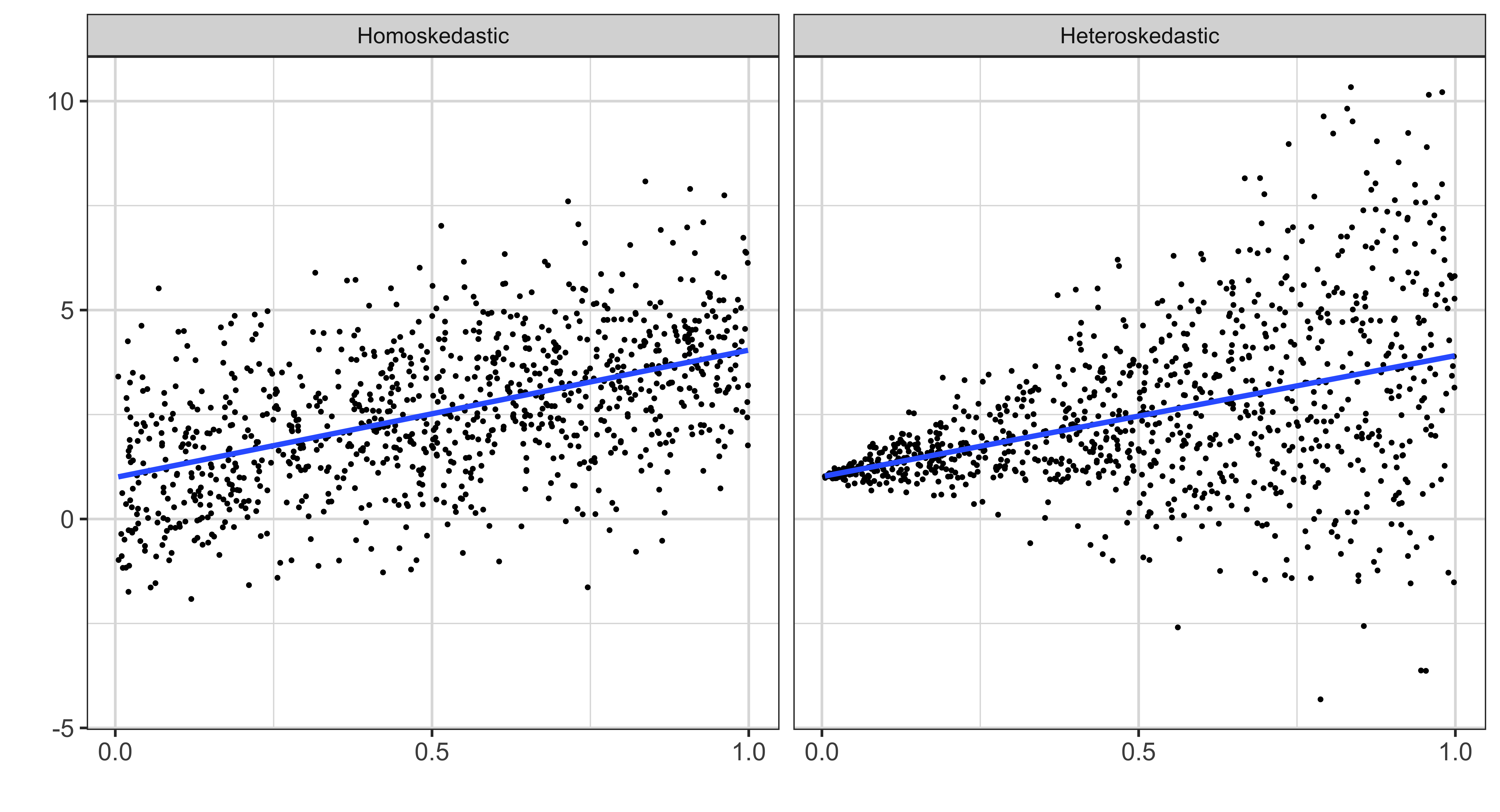
Two definitions, and the whole lecture turns on the difference between them. Start with the blue callout. Homoskedasticity says the variance of the error, conditional on x, equals sigma squared. Here, u is the unobserved error, x represents the explanatory variables we condition on, variance measures the spread of u around its conditional mean, and sigma squared is one constant positive number. The blue phrase underneath is the key: wherever you look in the x distribution, the conditional spread of the errors is the same.
Now compare the red callout. Under heteroskedasticity, that conditional variance is f of x. The letter f does not impose a particular formula. It simply says the error variance can change with x. For example, income prediction errors may spread out as education or experience rises. Heteroskedasticity concerns the variance, not the conditional mean. We can still have expected u given x equal to zero while the size of typical positive and negative errors changes.
Read the three bullets at the bottom for why this matters now. Constant conditional variance is MLR five, and every standard error, t-test, F-test, p-value, and confidence interval in lecture 05 used it. Normality gave it to us there because independence of u from x means the entire conditional distribution of u, including its variance, does not change with x. This lecture removes that protection.
Homoskedasticity
Var(u|x) = \sigma^2
Heteroskedasticity
Var(u|x) = f(x)
Read the difference: under homoskedasticity the spread of the error is the same number whatever x is. Under heteroskedasticity it is a function of x.
Look at the two panels. The horizontal axis is x, running from zero to one. The vertical axis is y, and each dot is one of one thousand simulated observations. Both panels were generated from the same conditional mean, one plus three times x, so the true intercept is one and the true slope is three. The blue line in each panel is the fitted OLS line through its cloud.
On the left, labeled Homoskedastic, the cloud has roughly the same vertical thickness at low, middle, and high values of x. The code generates those errors with a constant standard deviation of one point five, which is three times zero point five. On the right, labeled Heteroskedastic, the error standard deviation is three times x. Near x equals zero, the errors are therefore close to zero and the points hug the line. As x rises toward one, their standard deviation rises toward three, so the cloud opens into a fan. The upper and lower edges spread apart even though the middle stays on the same line.
This slide states the problem we are going to solve. Suppose reality is heteroskedastic, so the conditional error variance changes with x, but you proceed as if the errors were homoskedastic. There are two consequences to examine, and you must keep them separate.
The first bullet asks about estimating beta j itself. Beta hat j is an OLS coefficient estimate, such as the estimated slope on x. We want to know whether heteroskedasticity changes its expected value, creates bias, or otherwise invalidates OLS as a way to estimate the conditional mean relationship. That is a question about the center of the estimator’s sampling distribution.
The second bullet asks about estimating the variance of beta hat j. That variance describes how beta hat j would move across repeated samples. Its square root is the standard error, which is the denominator of a t-statistic and therefore feeds directly into p-values and confidence intervals. This is a question about the spread of the sampling distribution.
What are the consequences of assuming the error is homoskedastic when it is heteroskedastic in reality?
Take the first of the two central questions on its own. The screen asks whether OLS coefficient estimators remain unbiased when the error is heteroskedastic. Unbiased means that, over repeated random samples generated by the same process, the average value of beta hat j equals the true beta j.
Are OLS estimators unbiased when error is heteroskedastic?
Yes. The OLS coefficient estimator is still unbiased in the presence of heteroskedasticity, provided the assumptions that actually deliver unbiasedness, especially expected u given x equals zero, continue to hold. The sentence on screen gives the decisive reason: the proof of unbiasedness never used the homoskedasticity assumption.
Yes. We do not need to use the homoskedasticity assumption to prove that the OLS estimator is unbiased.
This tab reviews the familiar variance formula under homoskedasticity. On the first line, the variance of beta hat j equals sigma squared divided by S S T x times one minus R j squared. Sigma squared is the common conditional variance of the error. S S T x is the total sum of squares for the explanatory variable x j, so more sample variation in x j gives more information and lowers the coefficient variance. R j squared comes from the auxiliary regression of x j on all the other explanatory variables. When x j is highly explained by those variables, one minus R j squared is small, the denominator shrinks, and multicollinearity raises the variance of beta hat j.
Sigma squared is unknown, so the second line replaces it with sigma hat squared. Look at its definition: add the squared OLS residuals u hat i from observation one through N, then divide by N minus k minus one. N is the sample size, k is the number of slope regressors, and the additional one accounts for the intercept. Those lost degrees of freedom correct for estimating k plus one coefficients before measuring the remaining error variation.
The blue phrase in the callout is the operational point. R and other software use this homoskedastic formula by default. The reported standard error is the square root of the resulting estimated variance. Every default t-statistic, p-value, and confidence interval then inherits this assumption.
We learned that when the homoskedasticity assumption holds, then,
Var(\widehat{\beta}_j) = \frac{\sigma^2}{SST_x(1-R^2_j)}
We used the following as the estimator of Var(\widehat{\beta}_j)
\frac{\widehat{\sigma}^2}{SST_x(1-R^2_j)} where \widehat{\sigma}^2 = \frac{\sum_{i=1}^{N} \widehat{u}_i^2}{N-k-1}
Important
By default, R and other statistical software use this formula to get estimates of the variance of \widehat{\beta}_j.
But, under heteroskedasticity,
Var(\widehat{\beta}_j) \ne \frac{\sigma^2}{SST_x(1-R^2_j)}
Under heteroskedasticity, the line above this question tells you that the true variance of beta hat j is not sigma squared divided by S S T x times one minus R j squared. There is no single sigma squared that describes every observation’s conditional error variance. The question now asks whether the estimator built from that formula might nevertheless work on average.
Read the expression from left to right. Var hat of beta hat j, subscript default, denotes the variance estimate produced by the conventional homoskedastic formula. The triple-bar definition says that this object is sigma hat squared divided by S S T x times one minus R j squared. The outer expectation asks for the average value of that default estimator across repeated samples. On the right is the actual sampling variance of beta hat j.
So the equality asks whether the default estimator is unbiased for the true coefficient variance when errors are heteroskedastic. This is not the same as asking whether beta hat j itself is unbiased. We already answered that question yes. Here we are testing whether the estimated spread around that correctly centered coefficient is itself correct. Answer before opening the next tab.
Is E[\widehat{Var(\widehat{\beta}_j)}_{default}] \equiv E\Big[\frac{\widehat{\sigma}^2}{SST_x(1-R^2_j)}\Big]=Var(\widehat{\beta}_j) under heteroskedasticity?
No. Once the conditional variance of u changes with x, the default homoskedastic estimator is not generally unbiased for the true variance of beta hat j. It treats every observation as though it had the same error variance, even though observations at different x values can contribute very different amounts of uncertainty to the estimated slope.
No.
So, what are the consequences of using \widehat{Var(\widehat{\beta}_j)}=\frac{\widehat{\sigma}^2}{SST_x(1-R^2_j)} under heteroskedasticity?
\;\;\;\;\downarrow
Your hypothesis tests will generally have the wrong rejection rate.
The blue sentence above this question gives the consequence: hypothesis tests will generally have the wrong rejection rate. That follows as a chain. A biased variance estimate gives a wrong standard error after taking its square root. The standard error sits in the denominator of the t-statistic, so the t-statistic is mis-scaled. Its reference distribution and critical value no longer deliver the rejection probability you intended. P-values and confidence intervals are wrong for the same reason.
The question asks what people mean when they say hypothesis testing is biased. Be careful with the vocabulary. A test is a decision rule, not a coefficient estimate, so its bias is not described by an expected estimate being above or below a parameter. Instead, evaluate its behavior over repeated samples when the null hypothesis is true.
At a five percent significance level, the test is designed to reject a true null five percent of the time. If its actual rejection probability is higher, it over-rejects and produces too many false positives. If the probability is lower, it under-rejects and has an overly conservative false-positive rate. Think in those repeated-sampling terms, then open the Answer tab.
What does it mean to have hypothesis testing biased?
Biased testing here means that you reject a null hypothesis more often or less often than the chosen significance level intends. At a five percent level, the repeated-sampling promise is conditional: among hypothetical repetitions in which H zero is true, about five percent should end in rejection. Such a rejection is a Type I error.
If the standard error is underestimated, it makes the absolute t-statistic too large because the denominator is too small. More statistics cross the critical values, p-values become too small, confidence intervals become too narrow, and the test over-rejects. You then announce effects that are statistically significant more often than the nominal level permits. If the standard error is overestimated, the chain reverses: t-statistics are too small, p-values are too large, confidence intervals are too wide, and the test under-rejects.
The answer on screen therefore says roughly that testing bias is rejection too often or too rarely relative to your intention. It is not enough that an individual decision happened to be right or wrong. We judge the procedure by its long-run rejection rate.
Roughly speaking, it means that you over-reject/under-reject the hypothesis than you intend to.
Let’s run MC simulations to see the consequence of ignoring heteroskedasticity.
Model
y = 1 + \beta x + u, where \beta = 0
Test of interest
Here is the Monte Carlo setup. The model is y equals one plus beta times x plus u, and the data-generating process fixes beta at zero. The intercept is one, x is the explanatory variable, and u is the error. Because beta is zero, x has no true effect on the conditional mean of y.
The test is two-sided. H zero says beta equals zero, while H one says beta is not zero. We will test at a five percent significance level. The question writes the relevant conditional probability explicitly: the probability that we reject H zero given that H zero is true. That is the Type I error probability, or size, of the test.
In this simulation H zero is not merely plausible. It is made true by construction in every generated dataset. That gives us a benchmark before any code runs. State that target before opening the answer. Without a benchmark, the Monte Carlo output is just a number; with it, the output tells us whether ignoring heteroskedasticity breaks the test.
If you test the null hypothesis at the 5\% significance level, what should be the probability that you reject the null hypothesis when it is actually true?
Pr(\text{reject} \;\; H_0|H_0 \;\; \text{is true})=?
The target probability is five percent. That is exactly what a five percent significance level is supposed to control: when H zero is true, the test should make a Type I error with probability zero point zero five.
Here beta really equals zero in every repetition. Therefore every rejection is a false positive, not evidence that the simulated x occasionally acquired a real effect.
5\%
These five bullets are the complete Monte Carlo recipe. First, generate a dataset from y equals beta zero plus beta one x plus u while setting beta one, the coefficient on x, equal to zero. We will make u heteroskedastic, but keep its conditional mean at zero. Second, estimate the regression in each generated dataset. Save beta hat one, the estimated coefficient on x, and se hat of beta hat one, the estimated standard error. Third, calculate the t-statistic as beta hat x minus the null value zero, all divided by the estimated standard error of beta hat x. Because the null value is zero, the numerator simplifies to beta hat x. Reject the two-sided null when the absolute t-statistic exceeds the appropriate critical value.
Fourth, repeat data generation, estimation, and testing one thousand times. Each iteration is a fresh realization of the error, so the coefficient and t-statistic change even though the true parameter never does. Finally, count the rejections. About fifty out of one thousand would be consistent with the intended five percent size.
y=\beta_0+\beta_1 x + u
There are two code blocks here. The first is browser infrastructure. The context setup option makes it run once to prepare later WebR cells rather than present it as a separate exercise. The lecture-theme function starts from theme B W with a configurable base text size. The nested theme call scales axis text, axis titles, legend text, and the legend title; makes the plot, panel, legend, and legend-key backgrounds transparent; and restores visible gray grid lines against the deck’s warm background. WebR draws at seventy-two dots per inch even though the deck requests two hundred sixteen, so web r scale is three. The two assign-in-namespace calls scale ggplot’s point and stroke conversion constants, and theme lecture then uses an eighteen-point base multiplied by three. The final line and rectangle settings prevent that scaling from making borders nine times too thick. Theme set makes this the default for later browser plots. None of that changes the econometrics; it makes the interactive graphics match the rest of the deck.
The second block is the simulation itself. Set seed fixes the random-number stream so the class can reproduce the same result. N equals one thousand observations per dataset, B equals one thousand repetitions, and the two rep calls preallocate storage for coefficient estimates and t-statistics. The critical value uses q t at zero point nine seven five with N minus two degrees of freedom. We use zero point nine seven five because a two-sided five percent test leaves two point five percent in each tail, and subtract two degrees of freedom because this simple regression estimates an intercept and one slope.
The runif call draws x between zero and one once, outside the loop, so the same x values are held fixed across repetitions. Within each iteration, rnorm draws N standard-normal quantities with mean zero and observation-specific standard deviation two times x; multiplying by three makes the error standard deviation six times x. That is the line that creates heteroskedasticity: observations near zero have little error dispersion and those near one have much more. Then y equals one plus the error. There is deliberately no x term, so the true slope is zero.
Data frame combines y and x, and lm estimates y on an intercept and x. The dollar coef extraction selects the slope named x. Dee-tee bracket i stores it in the ith position. Vcov with no robust option returns the default homoskedastic variance-covariance matrix. The expression vcov underscore ols bracket x comma x selects the estimated variance of the x coefficient, square root turns that variance into a standard error, and beta hat divided by that standard error creates the t-statistic. We are therefore applying the default formula to data designed to violate it. Flip to Results to see whether the nominal five percent test keeps its promise.
The first line turns every stored t-statistic into a rejection decision. Abs takes the absolute value because this is a two-sided test, and the greater-than comparison asks whether that value exceeds the critical value. The result is a logical vector, TRUE for rejection and FALSE for non-rejection. Mean treats TRUE as one and FALSE as zero, so the mean of that vector is the fraction of simulations that rejected.
With the displayed seed and current R implementation, the output is zero point one zero eight, or ten point eight percent, which the callout rounds to about eleven percent. The target was five percent. Because beta is exactly zero in every generated dataset, every one of those rejections is a Type I error. This procedure produces false positives more than twice as often as its nominal level promises.
Now trace the mechanism in the callout. Over-rejection means too many absolute t-statistics crossed the critical value. Since each t-statistic is beta hat divided by its estimated standard error and the coefficient estimates remain unbiased, the systematic inflation comes from a denominator that is too small. A standard error that is too small is the square root of an estimated variance that is too small. In this particular design, therefore, the default formula underestimates the true variance of the OLS slope. Open the embedded Answer to confirm that chain. The final bullet is essential: under heteroskedasticity in general, the bias can go either direction.
Consequence of ignoring heteroskedasticity
We rejected the null hypothesis 10.8% of the time, instead of 5\%.
So, in this case, you are more likely to claim that x has a statistically significant impact than you are supposed to.
The use of the formula \frac{\widehat{\sigma}^2}{SST_x(1-R^2_j)} seemed to (over/under)-estimate the true variance of the OLS estimators?
The first sentence summarizes the failure we have established. Under heteroskedasticity, sigma hat squared divided by S S T x times one minus R j squared is a biased estimator of the sampling variance of beta hat. Because its square root supplies the standard error, tests, p-values, and confidence intervals based on it are not correctly calibrated. The question asks whether we can credibly estimate the coefficient variance without restoring homoskedasticity. The important callout answers yes. The White-Huber-Eicker estimator, named for the researchers associated with its development, produces what we call a heteroskedasticity-robust variance estimator and robust standard errors.
Focus on the red phrase, unknown form. We do not need to specify whether the error variance grows linearly with x, quadratically with x, differs by category, or follows the fan shape from the figure. We also do not need to estimate that variance function observation by observation.
Now, we understand the consequence of heteroskedasticity:
\frac{\widehat{\sigma}^2}{SST_x(1-R^2_j)} is a biased estimator of Var(\widehat{\beta}), which makes any kind of testings based on it invalid.
Can we credibly estimate the variance of the OLS estimators?
White-Huber-Eicker heteroskedasticity-robust standard error estimator
This slide displays one scalar form of the heteroskedasticity-robust variance estimator for beta hat j. Read the numerator as a sum from observation one through n of r hat i j squared times u hat i squared. U hat i is the OLS residual from the original regression of y on all explanatory variables. It estimates the unobserved error for observation i, so u hat i squared supplies an observation-specific measure of error variability rather than forcing one common sigma hat squared on everybody.
R hat i j comes from a separate auxiliary regression: regress x j on all the other explanatory variables and take observation i’s residual. That residual is the part of x j not explained by the other regressors, so it is the variation that identifies beta j. Squaring r hat i j weights observations according to how much identifying variation they contribute. An observation matters especially for the coefficient variance when it combines a large original residual, u hat i squared, with a large residualized x value, r hat i j squared.
The denominator is S S R j squared. The slide defines S S R j as the sum over i of r hat i j squared from that auxiliary regression. Then the entire sum is squared in the variance formula. Do not confuse the square on S S R j with merely summing fourth powers. First add the r hat squares, then square that total. The square root of the displayed variance estimate is the heteroskedasticity-robust standard error.
The note tells you we will not derive this estimator. Your required takeaways are the three bullets below it. Understand that heteroskedasticity invalidates the default uncertainty formula while leaving the OLS coefficients unbiased. Know that a robust, large-sample-consistent variance estimator exists for heteroskedasticity of unknown form. Finally, know how to request it in R or other statistical software.
Heteroskedasticity-robust standard error estimator
\widehat{Var(\widehat{\beta}_j)} = \frac{\sum_{i=1}^n \widehat{r}^2_{i,j} \widehat{u}^2_i}{(SSR_j)^2}
Note
We spend NO time to try to understand what’s going on with the estimator.
What you need is
This is the applied workflow. First, estimate the conditional mean model with OLS exactly as usual. You do not transform y, reweight the observations, or fit a different set of coefficients merely because the errors may be heteroskedastic. Under zero conditional mean, the OLS beta hats remain unbiased.
Second, assume the error can be heteroskedastic and estimate the variance-covariance matrix of those OLS coefficients with a heteroskedasticity-robust method. A variance-covariance matrix contains each coefficient variance on its diagonal and covariances between different coefficient estimates off the diagonal. The robust standard errors are the square roots of its diagonal entries.
The indented bullets mention the Breusch-Pagan and White tests, which test homoskedasticity against forms of heteroskedasticity. In practice, almost nobody needs to make robust inference conditional on first passing one of these tests, and we will not learn their R commands here. The reason is decision-theoretic: in a large sample, you would use robust standard errors whether or not a preliminary test detects heteroskedasticity. Testing first adds another uncertain decision without changing the final recommendation.
Third, use the robust variance estimates instead of the default homoskedastic estimates for inference. That means robust standard errors in t-statistics, robust p-values, robust confidence intervals, and robust joint tests. The final bullet prevents the common mistake: do not replace the coefficient estimates. Only the reported uncertainty and the conclusions that depend on it change.
Here is the well-accepted procedure in econometric analysis:
Estimate the model using OLS (you do nothing special here)
Assume the error term is heteroskedastic and estimate the variance of the OLS estimators
Replace the estimates from \widehat{Var(\widehat{\beta})}_{default} with those from \widehat{Var(\widehat{\beta})}_{robust} for testing
But, we do not replace coefficient estimates (remember, coefficient estimation is still unbiased under heteroskedasticity)
We now move from the formula to the R workflow using the M L B one dataset from the wooldridge package. The data call asks R to load the object named M L B one specifically from that package. The autorun option means this browser cell executes when the slide deck loads, so the regression object will already exist when you run the cells on the following tabs. The cell prints nothing because both lines assign objects rather than request output.
The regression call uses fixest double-colon feols. The double colon explicitly selects feols from the fixest package. Inside the formula, log of salary is the dependent variable. Taking the natural logarithm lets slope coefficients be interpreted approximately as proportional salary changes. Years in the league and batting average, abbreviated bavg, are the two explanatory variables, and feols includes an intercept by default. The data argument tells the function to find those variables in M L B one.
The result is assigned to reg underscore M L B for reuse. We have estimated ordinary OLS coefficients and left their stored inference at the default.
Let’s run a regression using the mlb1 data from the wooldridge package.
This slide gives you three ways to consume robust uncertainty. Stats double-colon vcov returns the complete variance-covariance matrix. Its diagonal entries are estimated coefficient variances and its off-diagonal entries are estimated covariances between coefficient estimators. Fixest double-colon se returns only the standard errors, which are the square roots of those diagonal entries. Summary uses the selected variance estimator to report coefficient tests of H zero colon beta j equals zero, including the standard error, t-statistic, and p-value.
Read the general syntax block. The first argument, labeled regression result, is a fitted model object such as reg underscore M L B. The named vcov argument selects the type of variance-covariance estimator. In real code, replace the placeholder string type of vcov with a supported choice. The second call has the same two inputs but returns only the standard-error vector. The namespace prefix on fixest double-colon se makes clear which package supplies se, which avoids ambiguity with functions of the same short name.
Now run the concrete browser cell. Vcov of reg underscore M L B with vcov equal to the string hetero returns the White-Huber-Eicker heteroskedasticity-robust matrix. Fixest se with the same model and same vcov choice returns robust standard errors for the intercept, years, and bavg. The quoted word hetero is doing all of the statistical work that differs from the default call. It tells fixest not to assume one common conditional error variance. The OLS model and its coefficients are not re-estimated.
We use
the stats::vcov() function to estimate heteroskedasticity-robust standard errors
the fixest::se() function from the fixest package to estimate heteroskedasticity-robust standard errors (you can always get SE from VCOV)
the summary() function to do tests of \beta_j = 0
General Syntax
Here is the general syntax to obtain various types of VCOV (and se) estimates:
heteroskedasticity-robust standard error estimation
Specifically for White-Huber heteroskedasticity-robust VCOV and se estimates,
Run the Default cell first. Se of reg underscore M L B has no vcov override, so it extracts the conventional homoskedastic standard errors. The parentheses around the assignment make R both save the vector as se underscore hom and print it. In the displayed dataset, the values are about zero point three four three for the intercept, zero point zero one three two for years, and zero point zero zero one three four for batting average.
Now run the Heteroskedasticity-robust cell. It uses the same fitted model but adds vcov equal to hetero, saves the result as se underscore het, and prints it. Those standard errors are about zero point seven zero four, zero point zero one seven seven, and zero point zero zero two nine eight. Compare term by term: all three robust values are larger in this application, the intercept and batting-average standard errors a little more than double, and the years standard error rises by roughly one third.
Default
Heteroskedasticity-robust
This slide shows how to report both uncertainty choices in a publication-style table. The first two lines compute and save the robust and homoskedastic variance-covariance matrices from the same reg underscore M L B object. Vcov underscore het adds vcov equal to hetero; vcov underscore homo leaves the default unchanged.
Modelsummary double-colon msummary receives a list containing the same fitted model twice, which creates two table columns with identical coefficient estimates. Its vcov argument receives a second list in matching order: the robust matrix for column one and the default matrix for column two. This one-to-one ordering matters. If the lists were reversed, the column labels in your explanation would be wrong. Stars equal TRUE asks modelsummary to add significance markers based on each column’s p-values. Gof underscore omit supplies a regular-expression string that removes fit rows whose names contain I C, Log, Adj, F, Pseudo, or Within, leaving a more compact table. The comment says to keep those presentation options unchanged.
Read the rendered table on the right by comparing each row across columns. Every coefficient is identical because both columns use the same OLS fit: the intercept is about eleven point zero four, the years coefficient about zero point one six six, and the bavg coefficient about zero point zero zero five four. The numbers in parentheses are the standard errors, and every pair differs because column one is robust while column two is conventional. For bavg, the default standard error is about zero point zero zero one three four, producing a t-statistic near four point zero four and three stars. The robust standard error is about zero point zero zero two nine eight, producing a t-statistic near one point eight one, a p-value around zero point zero seven one, and only a plus. Batting average moves from strong conventional significance to marginal significance solely because we stopped assuming homoskedasticity.
In presenting the regression results in a nicely formatted table, we used modelsummary::msummary().
We can easily swap the default se with the heteroskedasticity-robust se using the vcov option in msummary().
| (1) | (2) | |
|---|---|---|
| + p < 0.1, * p < 0.05, ** p < 0.01, *** p < 0.001 | ||
| (Intercept) | 11.042*** | 11.042*** |
| (0.704) | (0.343) | |
| years | 0.166*** | 0.166*** |
| (0.018) | (0.013) | |
| bavg | 0.005+ | 0.005*** |
| (0.003) | (0.001) | |
| Num.Obs. | 353 | 353 |
| R2 | 0.367 | 0.367 |
| RMSE | 0.94 | 0.94 |
| Std.Errors | Custom | Custom |
Column (1) uses the robust VCOV, column (2) the default. Read down the two columns:
bavg falls from *** to +: batting average goes from overwhelmingly significant to marginal purely because we stopped assuming homoskedasticityThis is the recommended implementation because it records the inference choice inside the fitted model object. Reg underscore M L B with r vcov is assigned the result of fixest double-colon feols. The formula is still log salary on years and bavg, so the OLS coefficients are the same as before. The data argument still points to M L B one. The only new argument is vcov equal to hetero, which tells fixest to attach the heteroskedasticity-robust variance-covariance estimator to the result.
The second call passes a one-element list containing that model to modelsummary double-colon msummary. There is no vcov list this time and no separate statistic override. Msummary reads the robust inference already stored in the object. Stars equal TRUE again adds significance markers, and gof underscore omit again removes the listed goodness-of-fit rows. The left code block hides its textual result because the formatted output is displayed in the right column, where echo is false so you see the table without duplicate code.
The statistical result is the same robust column you just constructed manually. The advantage is reliability, not a new estimator. Once vcov equal to hetero is set in feols, downstream summaries, tables, confidence intervals, and coefficient tests use that choice automatically. It still does not alter the coefficient estimates; it changes the variance information stored with them.
Alternatively, you could add the vcov option like below inside fixest::feols(). Then, you do not need statistic_override option to override the default VCOV estimates.
| (1) | |
|---|---|
| + p < 0.1, * p < 0.05, ** p < 0.01, *** p < 0.001 | |
| (Intercept) | 11.042*** |
| (0.704) | |
| years | 0.166*** |
| (0.018) | |
| bavg | 0.005+ |
| (0.003) | |
| Num.Obs. | 353 |
| R2 | 0.367 |
| RMSE | 0.94 |
Now we validate the robust estimator with the same Monte Carlo logic used to expose the default estimator. The opening question is empirical: does this method bring the rejection probability back toward the nominal five percent level when the errors are heteroskedastic?
Set seed fixes a new reproducible random stream. The code uses N, B, beta-hat storage, t-stat storage, and the critical value already created earlier. Runif draws N x values between zero and one once before the loop, so x again stays fixed across repetitions. Inside the loop, rnorm draws N mean-zero errors with observation-specific standard deviation two times x, and the outer factor of three makes the standard deviation six times x. Y equals one plus that error, so the true coefficient on x remains exactly zero. Data frame packages y and x for estimation.
Feols estimates y on x by OLS. The coefficient extraction selects the element named x and stores it in beta hat store at position i. Up to this point the data-generating process and coefficient estimator have the same structure as the broken test. The highlighted line is the crucial change: se of ols underscore res with vcov equal to hetero requests the robust standard-error vector, and bracket x selects the standard error for the slope. The t-statistic divides the unchanged beta hat by this robust standard error and stores the result.
Because the null value is zero, no subtraction appears in the numerator. Because the only inferential change is the vcov choice, a corrected rejection rate can be attributed to the robust variance estimator rather than to a different model, different coefficients, or a different heteroskedastic pattern. Move to the results tab to make that comparison.
Does the heteroskedasticity-robust se estimator really work? Let’s see using MC simulations:
The code repeats the rejection calculation. Abs makes the stored t-statistics two-sided, the greater-than comparison checks them against the previously computed critical value, and mean converts the TRUE and FALSE decisions into a rejection proportion. With the displayed seed, the current run returns zero point zero five three, or five point three percent.
Compare all three quantities printed in the sentence below the cell. The robust procedure rejects about five point three percent of true nulls. The default procedure rejected about ten point eight percent. The target is five percent. Monte Carlo results are not expected to equal the target exactly in only one thousand repetitions, so a three-tenths-of-a-percentage-point difference is ordinary simulation noise. The large excess rejection seen with the default standard error is essentially gone.
The two bullets state the correct conclusion and its scope. The robust estimator is not magically perfect in every finite sample, but it restores approximately correct test size in this large-sample design. More importantly, nothing about coefficient estimation changed. We used the same form of heteroskedastic data, the same OLS objective, and the same beta hats. Only the formula estimating the sampling variance changed. That one replacement corrected the standard errors, which corrected the t-statistics and therefore the rejection decisions.
We reject 5.3% of the time, against the 10.8% we got with the default estimator and the 5% we are aiming for.
We now turn from unequal error variances to dependence across observations. The two bullets above the tabs define the setting: observations can often be grouped into clusters, and errors belonging to observations in the same cluster can be correlated. A cluster is a collection whose members share shocks or omitted characteristics. Errors may be dependent within a cluster while different clusters are treated as independent.
Example one groups students by college. The equation says college G P A equals beta zero plus beta one times income plus beta two times high-school G P A plus u. College G P A is the outcome. Income and high-school G P A are observed explanatory variables. The error u contains every determinant of college G P A omitted from the regression.
Suppose the sample contains students from many colleges and one omitted determinant is each college’s grading policy. Students at a lenient college may all receive college G P A values above what income and high-school G P A predict, giving many positive errors. Students at a strict college may all have negative errors. Two students at the same college therefore share a college-level component in u, so knowing one student’s error tells you something about another’s. The observations are not independent pieces of information. College is the natural cluster because that is the level at which the omitted grading environment is shared.
College GPA: cluster by college
GPA_{col} = \beta_0 + \beta_1 income + \beta_2 GPA_{hs} + u
Example two has the same dependence structure with individuals as the groups. The sample follows five hundred people for ten years, producing five thousand person-year observations. The outcome is income and education is an explanatory variable of interest. Repeated observations let us see the same person’s income at several points in time, but they do not create ten independent versions of that person.
The bullet identifies innate ability as an omitted individual characteristic. If ability affects income but is not completely represented by the regressors, it sits inside u. The same person’s ability is present in all ten years, so that person’s errors tend to move together over time. A positive unexplained income component this year makes a positive unexplained component next year more likely. The cluster is therefore the individual: all ten time-series observations for one person belong together.
Education Impacts on Income: cluster by individual
Your observations consist of 500 individuals with each individual tracked over 10 years
Because of some unobserved (omitted) individual characteristics, error terms for time-series observations within an individual might be correlated.
Question one repeats the estimation-versus-inference distinction. Does correlation among errors within a cluster make the OLS coefficient estimators biased? To answer, write the two kinds of correlation separately. Correlation between an explanatory variable x and the error u threatens the zero-conditional-mean assumption and can bias beta hat. Correlation between u i and u h for two observations in the same group describes dependence across errors.
Those are not the same statement. If expected u given the full set of x values is zero, the OLS estimator can still be centered on the true beta even when errors from classmates, people in the same village, firms in the same industry, or repeated observations of one individual move together. The answer hidden on the slide is therefore no: correlation among the u’s does not by itself bias OLS coefficients.
Are the OLS estimators of the coefficients biased in the presence of clustered error?
Question two asks whether the default estimator of the variance of beta hat remains unbiased in the presence of clustered errors. The hidden answer is no. The conventional formula relies on more than equal diagonal variances. It also relies on different observations’ errors having zero conditional covariance.
Picture the variance-covariance matrix of the error vector. Each diagonal entry is the variance of one observation’s error. Homoskedasticity makes those diagonal entries equal to sigma squared. Each off-diagonal entry is a covariance between two different observations’ errors. Independent sampling, together with the regression assumptions, makes those entries zero in the conventional derivation. Clustered error creates blocks of nonzero off-diagonal covariances for pairs belonging to the same group.
Those covariance terms enter the true sampling variance of OLS because beta hat is built from a weighted combination of all observations’ errors. The default estimator discards them as though every observation supplied an independent shock. Even perfectly constant marginal variances would not rescue it; homoskedasticity concerns the diagonal and does not imply zero off-diagonal covariance.
Are \widehat{Var(\widehat{\beta})}_{default} unbiased estimators of Var(\widehat{\beta})?
Start with the information question. Two independent errors carry more information than two positively correlated errors. If the second error is independent of the first, observing it supplies a genuinely new realization. If the two are strongly correlated, knowing the first lets you partly predict the second, so the second observation adds less new information. At the extreme, two identical errors are repetition of one shock, not two independent shocks.
Now apply that intuition to the first fill-in-the-blank. The default variance estimator behaves as though all observations are independent. With positive within-cluster correlation, it therefore counts more independent information than the sample truly contains. Greater presumed information implies greater presumed precision, so it tends to underestimate the true variance of beta hat. The hidden answer highlights under.
Move through the second blank as a causal chain. An underestimated variance produces an underestimated standard error after taking the square root. Dividing beta hat by a denominator that is too small produces an absolute t-statistic that is too large. Too many statistics cross the critical value, so you reject the null more often than intended. The hidden answer highlights more.
Which has more information?
Consequences
If you were to use \widehat{Var(\widehat{\beta})}_{default} to estimate Var(\widehat{\beta}) in the presence of clustered error, you would (under/over)-estimate the true Var(\widehat{\beta}).
This would lead to rejecting null hypothesis (more/less) often than you are supposed to.
The simulation again tests whether a nominal five percent procedure has the right rejection rate, but the data-generating process now violates independence rather than constant variance. The first bullet says to create clustered errors in two clusters in the conceptual illustration, while the code that follows uses fifty groups for a more informative experiment. In either case, observations inside a group share correlated components. The model is y equals beta zero plus beta one x plus u, and beta one is fixed at zero so the null is true.
For each generated dataset, estimate OLS and extract beta hat x together with its estimated standard error. Calculate the t-statistic as beta hat x divided by se hat of beta hat x. The subtraction of the null value is absent because that value is zero. Repeat data generation, regression, and t-statistic construction one thousand times. Then count how many absolute t-statistics reject H zero colon beta x equals zero. Because that null is true in every repetition, a correctly sized five percent test should reject around fifty times.
Here are the conceptual steps of the MC simulations to see the consequence of clustered error.
\begin{aligned} y = \beta_0 + \beta_1 x + u \end{aligned}
This cell builds one clustered dataset. N is two thousand total observations, G is fifty groups, and N g equals N divided by G, so each group contains forty observations. Those equal group sizes simplify the simulation.
For u, MASS double-colon mvrnorm generates G multivariate-normal draws. Its first argument, G, means one draw per group. Mu equals rep zero N g gives each forty-dimensional draw a vector of zero means. Sigma specifies the forty-by-forty covariance matrix. Matrix ten fills every entry with ten, and diag N g adds one only to the diagonal. Each error therefore has variance eleven, while every pair of distinct errors in the same group has covariance ten. Their correlation is ten divided by eleven, about zero point nine one, which is very strong. Different mvrnorm rows are drawn independently, so dependence is within groups but not across them.
The pipe sends the resulting fifty-by-forty matrix to t, making observations from the same group contiguous, then c flattens it into a vector of length two thousand. The x block repeats the construction independently. Its covariance matrix has ones everywhere and adds zero point two on the diagonal, so each x has variance one point two, pairwise within-group covariance one, and correlation about zero point eight three. Generating x independently of u keeps the true slope exogenous while making much of x’s identifying variation occur between groups.
Y is one plus zero times x plus u. Writing zero times x makes the true slope visually explicit even though the term contributes nothing. Finally, data frame binds y, x, and a group identifier. Rep one colon G, each equals N g repeats each group number forty times, matching the ordering created by transpose and flatten. The result has two thousand rows, fifty independent clusters, strongly correlated errors within each cluster, and a true coefficient on x of zero.
Run this plot and read both axes. The horizontal axis is group, with categories one through fifty. Factor of group tells ggplot to treat those numbers as discrete clusters rather than a continuous numeric scale. The vertical axis is y, the generated outcome. Geom point draws one dot per observation with y mapped vertically and the group factor mapped horizontally. Size zero point two keeps the forty points in each group from obscuring one another. X lab supplies the axis title group.
Theme lecture applies the deck’s common appearance. The additional theme call changes only the horizontal-axis labels: element text uses six times the WebR scale for readable rendered size and angle ninety rotates the fifty group numbers vertically so they do not overlap.
Each vertical strip contains the forty observations from one group. If errors were independent across all two thousand rows, the strips would look like comparable random samples from one common vertical band, with no persistent group-level displacement. Instead, whole strips sit unusually high or low because members share a large common error component. A group receiving a positive common shock moves many of its y values upward together; another group’s negative shock moves its column downward. That coordinated motion is what within-group error correlation looks like.
Do not infer that every dot within a group is identical. The identity component in the covariance matrix adds observation-specific noise, so there is still vertical spread inside each column. The figure separates the shared and individual pieces visually. It also shows why two thousand rows overstate the independent information: much of the movement occurs through only fifty group-level shocks.
This Monte Carlo cell puts the preceding data-generating process inside a loop. The label cluster M C names the cell. Set seed makes its random draws reproducible. B is one thousand repetitions, t stat store is a preallocated numeric vector of that length, and N, G, and N g again specify two thousand observations arranged as fifty groups of forty.
In each iteration, the two mvrnorm pipelines regenerate u and x. For u, G group-level multivariate draws have zero means, variances eleven, and within-group covariances ten. For x, the corresponding variances are one point two and covariances one. Transpose and c preserve contiguous group ordering. Y is reset to one plus zero times x plus u, and data frame combines the variables with group numbers repeated forty times each. Fresh u and x draws make each iteration a new dataset, while the true slope remains zero.
Feols estimates y on x by ordinary least squares. Notice what is missing: there is no cluster argument in this first experiment. Se of reg, bracket x, therefore selects the default standard error for the x coefficient, which treats all two thousand observations as independent. The next line extracts the x coefficient and divides it by that default standard error. Because the null value is zero, this is the test statistic directly. Dee-tee bracket i comma stores it for the ith repetition.
The code does not save beta hats separately because this experiment needs only the rejection behavior. It also does not use the group column during estimation, even though group is present in the data. That omission is deliberate: we are measuring what goes wrong when clustering is known in the data structure but ignored in inference. Each iteration draws two multivariate-normal samples, so the browser may take a moment. Predict whether the false-positive rate will be above or below the earlier eleven percent before opening Results.
The first line computes the two-sided critical value using q t at zero point nine seven five with N minus two degrees of freedom. Again, zero point nine seven five leaves two point five percent in the upper tail, and N minus two accounts for the intercept and slope in the simple regression. The next line takes absolute stored t-statistics, compares them with that critical value, and averages the logical decisions to obtain the rejection rate.
With the displayed seed, the result is zero point seven five one, or seventy-five point one percent. The correct null is being rejected about three times in every four, rather than one time in twenty. The coefficient on x is exactly zero in the data-generating process, and x was generated independently from u, so this is not evidence of a real effect or bias caused by endogeneity. It is catastrophic size distortion from the default standard error.
The callout explains the direction. Strong positive correlation makes forty rows within a group convey much less than forty independent errors would. Moreover, x is itself highly correlated within group, so the slope relies heavily on group-level comparisons. The default estimator ignores those shared shocks and acts as if N equals two thousand independent observations determined its precision. It therefore greatly underestimates the true variance and standard error, inflates the absolute t-statistics, and makes explanatory variables look far more significant than they are.
Important
The fix has the same structure as the heteroskedasticity repair. There are variance-covariance estimators that allow errors to have arbitrary correlation within a specified cluster while treating different clusters as independent. The slide denotes such an estimate by Var hat of beta hat, subscript c l. The diagonal elements estimate the variances of the coefficient estimators, and their square roots are cluster-robust standard errors.
The blue sentence says we will neither derive nor display the mathematical expression. What matters is knowing what dependence it permits and what information you must supply. Read every bullet in the note as a learning objective. First, understand the consequence: conventional standard errors can drastically understate uncertainty and make tests over-reject when positively correlated errors are ignored. Second, know that an appropriate variance estimator exists, so you do not have to abandon the OLS coefficients. Third, the estimator used here also permits heteroskedasticity within clusters. It is therefore both cluster-robust and heteroskedasticity-robust, so you do not apply a separate White-Huber correction on top of it. Fourth, know how to request it in R or other software. The next tabs supply that implementation.
There exist estimators of Var(\widehat{\beta}) that take into account the possibility that errors are clustered.
We call such estimators cluster-robust variance covariance estimator denoted as (\widehat{Var(\widehat{\beta})}_{cl})
We call standard error estimates from such estimators cluster-robust standard error estimates
I neither derive nor show the mathematical expressions of these estimators.
This is what you need to do
understand the consequence of clustered errors
know there are estimators that are appropriate under clustered error
know that the estimators we will learn take care of heteroskedasticity at the same time (so, they really are cluster- and heteroskedasticity-robust standard error estimators)
know how to use the estimators in R (or some other software)
The opening text connects this syntax to the heteroskedasticity case. We previously selected a robust estimator with the vcov option. For cluster-robust uncertainty, fixest accepts a cluster option that identifies the grouping variable.
Before estimating anything, inspect the data. Dplyr double-colon select takes M L B one as its first input and keeps only salary, years, bavg, and n l. The pipe passes that four-column table to head, which prints the first six rows by default. Salary is the outcome in levels before we take logs, years is time in the major leagues, bavg is batting average, and n l is the proposed group indicator.
The bullet defines n l exactly: one means the player is in the National League, and zero means the player is in the American League. Players with the same value would be treated as sharing potentially correlated errors. In syntax terms, n l is the variable around which we cluster.
Now count the distinct values. A binary indicator creates only two clusters, one per league.
Cluster-robust standard error
Similar with the vcov option for White-Huber heteroskedasticity-robust se, we can use the cluster option to get cluster-robust se.
Before an R demonstration
Let’s take a look at the MLB data again.
nl: the group variable we cluster around (1 if in the National league, 0 if in the American league).Step one estimates exactly the same OLS model as before. Autorun makes the browser execute the cell on load. Feols receives log salary as the dependent variable, years and bavg as regressors, and M L B one as the data source. The result is assigned to reg underscore M L B. There is no cluster option in this fitting call, so the object initially carries default inference, but its OLS coefficients are ready for either variance estimator.
Step two computes clustered uncertainty after estimation. Vcov receives the fitted model and cluster equal to tilde n l. The tilde is important: this is a one-sided formula telling fixest to find n l in the model’s original data and use its values as cluster identifiers. Vcov returns the complete cluster-robust variance-covariance matrix. The following se call uses the same cluster formula but returns only the square roots of the diagonal entries.
The model coefficients do not change between these calls. The cluster option changes how residual contributions are aggregated when estimating their sampling variance. Observations with the same n l value are allowed arbitrary heteroskedasticity and covariance; the two leagues are treated as independent clusters. This mirrors the earlier post-estimation syntax vcov equal to hetero, so the workflow is easy to transfer.
Step 1
Run a regression
Step 2
Apply vcov() or se() with the cluster = option.
The top cell calls se of reg underscore M L B with no override. It returns the default homoskedastic standard errors for the intercept, years, and batting average, treating player-level errors as uncorrelated. The lower cell uses the same fitted model but adds cluster equal to tilde n l. It returns cluster-robust standard errors that permit all players in the same league to share arbitrary error covariance and heteroskedasticity.
Compare the two vectors term by term rather than looking for a universal direction. The clustered values differ from the defaults because within-league residual co-movement is now included.
Default
Cluster-robust standard error
This is the recommended way to store the clustering decision. The general syntax puts cluster equal to tilde variable to cluster by directly inside fixest double-colon feols. The formula y tilde x specifies the regression, and data tells feols where both the regression variables and cluster identifier live. The eval false option marks this first block as a syntax template rather than executable code.
The concrete example assigns reg underscore M L B to feols of log salary on years and bavg. Cluster equal to tilde n l identifies league membership as the grouping level, and data equal to M L B one supplies all variables. Feols still computes the ordinary OLS coefficient estimates. It also stores the cluster-robust variance choice with the model object.
Tidy of reg underscore M L B then returns one row per coefficient with the estimate and its attached inferential quantities, including clustered standard errors, test statistics, and p-values. No cluster option needs to be repeated because tidy reads the model’s stored vcov specification.
Or, you could add the cluster option inside fixest::feols().
Syntax
Example
This code cluster by nl.
This slide turns the cluster discussion into an applied procedure. First, estimate the conditional mean model using OLS without changing the coefficient computation. Under the maintained exogeneity assumptions, within-cluster error correlation does not itself bias beta hat.
Second, allow the errors to be clustered and heteroskedastic when estimating Var of beta hat. Supply a defensible cluster identifier and use the cluster-robust variance-covariance estimator. Third, replace the default variance estimates with Var hat of beta hat subscript c l for inference. Take their diagonal square roots for cluster-robust standard errors, then use those values in t-statistics, p-values, confidence intervals, and joint tests. Because the estimator used here also handles heteroskedasticity, do not layer a separate heteroskedastic correction over it.
Finally, do not replace the coefficient estimates. The fitted model, beta hats, and predictions remain OLS. Only their estimated uncertainty changes. This is deliberately parallel to the earlier workflow: heteroskedasticity changes diagonal error variances, clustering adds within-group covariance, and each violation breaks the default uncertainty formula without automatically breaking OLS coefficients.
Just like the heteroskedasticity-present case before,
Estimate the model using OLS (you do nothing special here)
Assume the error term is clustered and/or heteroskedastic, and estimate the variance of the OLS estimators (Var(\widehat{\beta})) using cluster-robust standard error estimators
Replace the estimates from \widehat{Var(\widehat{\beta})}_{default} with those from \widehat{Var(\widehat{\beta})}_{cl} for testing
But, we do not replace coefficient estimates.
Let’s run MC simulations to see if the use of the cluster-robust standard error estimation method works
This is the direct repair experiment. Set seed, B, N, G, and N g reproduce the earlier design: one thousand simulations, two thousand observations, fifty groups, and forty observations per group. T stat store is reset so the new experiment does not mix its statistics with the default-standard-error run.
Inside each iteration, mvrnorm again creates strongly correlated within-group errors with variance eleven and covariance ten, and correlated within-group x values with variance one point two and covariance one. Transpose and c arrange the group members contiguously. Y equals one plus zero times x plus u, and the group column repeats each identifier N g times. The true x coefficient is still zero and x is still generated independently of u.
The highlighted feols line is the only statistical repair. It estimates y on x from data but now adds cluster equal to tilde group. The OLS coefficient is unchanged; the fitted object carries a variance estimator that aggregates residual score contributions at the group level and permits heteroskedasticity and arbitrary correlation within each group. Se of reg bracket x therefore retrieves the cluster-robust standard error rather than the default. Dividing the x coefficient by it produces the t-statistic, which is stored at position i.
The critical-value calculation now uses q t at zero point nine seven five with G minus one degrees of freedom. The two-sided tail probability is unchanged, but the reference degrees of freedom follow the number of independent clusters rather than the two thousand rows. With fifty groups, G minus one is forty-nine. The next line compares the absolute cluster-robust t-statistics with that critical value and averages the rejection indicators.
Read the numerical result produced by the cell and compare it with both benchmarks. It is in the single digits for this fixed-seed design, a different world from the seventy-five point one percent rejection rate under default standard errors, but still not guaranteed to equal the five percent target. The main conclusion does not depend on treating that Monte Carlo approximation as an exact constant: accounting for clustering removes most of the catastrophic size distortion, while a finite number of groups can leave noticeable error.
The callout explains why. Cluster-robust inference improves as the number of independent groups grows. It is asymptotic in G, not simply in the row count N. Two thousand observations arranged into fifty correlated blocks do not provide the same inferential foundation as two thousand independent groups. That is also why the M L B example’s two leagues are plainly insufficient. At the same time, no universal cluster count guarantees accurate inference. Leverage, group-size balance, influential clusters, and within-group dependence strength all matter. Treat fifty as an illustration of major improvement, not as a certification threshold.
Well, we are still rejecting more often than we should, but it is a different world from the 75.1% we got with the default estimator.
Important
This simulation keeps the same null hypothesis, dependence structure, estimator, and one thousand Monte Carlo repetitions, but greatly increases the number of independent groups. N is now twenty thousand, G is one thousand, and N g equals twenty observations per group. Increasing N alongside G keeps group size manageable while giving the cluster-robust approximation many more independent cluster contributions.
The two mvrnorm calls retain the same covariance structures. Within each group, u has variance eleven and pairwise covariance ten, while x has variance one point two and pairwise covariance one. Y remains one plus zero times x plus u, and data frame assigns twenty consecutive observations to each group. Feols estimates the same zero-slope regression with cluster equal to tilde group. Se of reg bracket x retrieves the attached cluster-robust standard error, and each slope divided by that value is stored as a t-statistic.
The note warns about computation. Each of one thousand iterations now fits a regression to twenty thousand observations and constructs multivariate draws for one thousand groups. Desktop R takes roughly half a minute in the environment used for the slide, while WebR in the browser can take several minutes. A long wait is expected behavior, not evidence that the cell has hung.
Conceptually, this is a diagnostic for the approximation. If the remaining distortion with fifty groups came from having too few independent clusters, increasing G from fifty to one thousand should move the rejection rate closer to five percent. If the robust formula were addressing the wrong dependence structure, simply adding groups would not systematically help. Flip to Results only after stating that prediction.
The only change from the previous simulation is G: 1000 groups instead of 50.
This one takes a while
1000 iterations on 20,000 observations runs in about half a minute in desktop R, so expect a few minutes in the browser. It has not hung.
The results code uses q t at zero point nine seven five with G minus one degrees of freedom. With one thousand groups, that is nine hundred ninety-nine degrees of freedom and the critical value is very close to the standard-normal value one point nine six. Abs makes the test two-sided, the comparison creates rejection indicators, and mean reports their proportion.
The result is closer to the five percent target than the corresponding fifty-group experiment, which supports the large-number-of-clusters explanation. It is still a Monte Carlo proportion from one thousand repetitions, so exact equality with zero point zero five is neither expected nor required. Sampling noise in the experiment and finite-sample behavior of the estimator both remain.
The sentence below the cell summarizes the intended comparison: increasing the number of groups improves the test, and using cluster-robust inference is certainly better than the default procedure that rejected roughly seventy-five percent of true nulls. Do not turn that into a guarantee that cluster-robust standard errors are exact. Their conventional justification is asymptotic as the number of independent groups grows.
Better. But, we are still over-rejecting. Don’t forget it is certainly better than using the default!
This table compresses both halves of the lecture, so read each row across the two columns. In the first row, heteroskedasticity means Var of u conditional on x depends on x. Clustered error means distinct observations’ errors are correlated within a group. These violate different pieces of the usual error variance-covariance structure: unequal diagonal variances in the first case, nonzero within-group off-diagonal covariances in the second.
The beta hat j row is blue in both columns because OLS coefficients remain unbiased under the maintained zero-conditional-mean assumptions. Neither violation by itself requires changing the fitted coefficients. The next row says the default variance estimator is biased in both cases, often severely under clustering. Therefore the downstream standard errors, t-statistics, p-values, and confidence intervals from lecture 05 are what break.
The first rejection-rate row reports the illustrative simulations. At a nominal five percent level, the heteroskedastic design rejected about eleven percent of true nulls, while the clustered design using defaults rejected about seventy-five percent. In these data-generating processes, ignored clustering creates the larger distortion. That ranking is not universal; it depends on where heteroskedasticity appears, how strong within-group correlation is, how x varies, and the leverage structure.
The fix row gives the one-argument implementations in feols. Use vcov equal to hetero for general heteroskedasticity, or cluster equal to tilde group when dependence occurs within a defensible grouping. The last row records approximately five percent after the heteroskedasticity repair and approximately nine percent in the deck’s fifty-group clustered summary. Those are Monte Carlo outcomes, not universal performance guarantees. The common three-step story is: preserve OLS coefficients, replace the invalid variance estimator, and redo every inferential quantity using the robust standard errors.
Heteroskedasticity and clustered errors violate different parts of the usual error variance-covariance structure, but the practical response is similar:
| Heteroskedasticity | Clustered error | |
|---|---|---|
| What breaks | Var(u\|x) depends on x | errors are correlated within a group |
| \widehat{\beta}_j | still unbiased | still unbiased |
| \widehat{Var(\widehat{\beta}_j)}_{default} | biased | biased, usually badly |
| Rejection rate at the 5% level | ~11% | ~75% |
| The fix | vcov = "hetero" |
cluster = ~ group |
| Rejection rate after the fix | ~5% | ~9% |
End with four working rules. First, use heteroskedasticity-robust standard errors by default in large samples. They protect inference against heteroskedasticity of unknown form, so you do not have to guess the variance function. In finite samples they can differ from conventional standard errors even when homoskedasticity happens to hold. Robust means valid under a broader set of conditions asymptotically, not identical and costless in every finite sample. In feols, the implementation is the single argument vcov equal to hetero.
Second, if errors can be correlated within groups, cluster at a defensible level. Let the data collection, shared shocks, or treatment-assignment process guide the choice. If treatment is assigned to schools, villages, firms, or states, clustering at that assignment level is a common starting rule because observations receiving a shared treatment can share errors. A variable with only two groups, such as league in the M L B demonstration, is not enough for conventional cluster-robust inference. You need many independent groups, not merely many rows within each group.
Third, do not make robust inference conditional on first running a Breusch-Pagan or White test. Those tests exist, but a noisy preliminary decision does not help when your large-sample practice would use heteroskedasticity-robust standard errors either way. Fourth, never swap the coefficient estimates. The OLS beta hats stay fixed; only their estimated standard errors and the tests, p-values, and intervals built from them change.
Finally, read the callout as the limitation connecting this lecture to lecture 08. Both robust estimators are asymptotic. Heteroskedasticity-robust inference improves as the sample grows, while conventional cluster-robust inference needs the number of independent groups to grow. With fifty groups the slide records rejection around nine percent rather than five, and with one thousand groups it improves again. These methods are protections, not finite-sample guarantees. Lecture 08 develops the large-sample arguments that justify using them.
Use heteroskedasticity-robust standard errors by default in large samples. They protect inference against unknown heteroskedasticity. In finite samples they can differ from conventional standard errors even when the errors are homoskedastic, so “robust” does not mean literally costless. The hetero option in feols() is one argument.
If errors may be correlated within groups, cluster at a defensible level. The choice should follow the sampling or treatment-assignment process; clustering at the level at which treatment is assigned is a common rule of thumb. Clustering by a group with only two levels, as in the MLB league example, is not enough — you need many groups for conventional cluster-robust inference to behave well.
Do not test for heteroskedasticity first. The tests exist (Breusch-Pagan, White), but almost nobody runs them, because the answer changes nothing: you would use robust standard errors either way.
Never swap the coefficients. Only the standard errors change.
Why cluster-robust was still over-rejecting
Both robust estimators are asymptotic: they are correct as the sample (or the number of groups) grows, not in any finite sample. With 50 groups we rejected about 9% instead of 5%; with 1000 groups it improved again. That is a preview of lecture 08, where large-sample arguments replace the exact finite-sample results we have been relying on.