05: Hypothesis Testing
Hypothesis Testing
Transcript
Every test in this lecture follows these same five steps, so use this slide as a map. Step one is to state the null hypothesis, H zero, and the alternative, H one. The null is the claim you subject to a test; the alternative describes the departure that would make you reject it.
Step two is the intellectual core. Choose a test statistic and find its sampling distribution under the assumption that H zero is true. The red phrase matters twice on this slide. We are not asking for the statistic’s distribution under every possible state of the world. We temporarily impose the null so that we have a reference distribution against which an observed result can be judged. If you do not know that null distribution, you do not yet have a formal test.
In step three, calculate the statistic from your sample and regression output. In step four, choose the significance level, such as five percent. That is the long-run Type I error rate you are willing to tolerate, and it determines a rejection region or critical value. Finally, in step five, ask how unusual the statistic from step three would be in the null distribution from step two. If it is sufficiently extreme, you reject H zero in favor of H one. If it is not, you fail to reject H zero. You do not prove the null true.
Here is the general step of any hypothesis testing:
Step 1: specify the null (H_0) and alternative (H_1) hypotheses
Step 2: find the distribution of the test statistic if the null hypothesis is true
Step 3: calculate the test statistic based on the data and regression results
Step 4: define the significance level
Step 5: check how unlikely that you get the actual test statistic (found at Step 3) if indeed the null hypothesis is true
Transcript
This is a deliberately artificial example, and the artificiality lets us see the testing logic without having to estimate a variance first. The goal at the top says that x is Normally distributed and that we want to test whether its population expected value is one. I will call the unknown population mean alpha. The phrase “or not” makes this a two-sided question: values of alpha either above or below one would count against the null.
The state of knowledge gives us unusually strong information. We know the population distribution is Normal and we somehow know its variance is four, so its standard deviation is two. In real applications, a population variance is almost never handed to us.
Our estimator is theta, the sample mean. Read the formula as theta equals the sum of x sub i from i equals one through J, divided by J. Here J is the number of observations, x sub i is observation i, alpha is the population mean we want to learn about, and theta is the random estimator computed from whichever sample we happen to draw. From the earlier lecture, you know theta is unbiased, so its expected value is alpha. But one observed sample mean will almost never equal alpha exactly. The testing question is therefore not simply whether theta equals one. It is whether theta is far enough from one, relative to its sampling variation, that the discrepancy would be hard to explain if alpha really were one. Flip to the distribution tab to quantify that sampling variation.
Goal
Suppose you want to test if the expected value of a normally distributed random variable (x) is 1 or not.
State of Knowledge
We do know x follows a normal distribution and its variance is 4 for some reason.
Your Estimator
Your estimator is the sample mean: \theta = \sum_{i=1}^J x_i/J
Transcript
Follow the two math asides carefully, because together they produce the statistic we will test. Math Aside 1 says that if you multiply a random variable X by a constant a, its variance is multiplied by a squared. This is why standard deviations scale by the absolute value of a. Math Aside 2 says that subtracting a constant shifts a Normal distribution’s mean but does not change its variance. Thus, if x follows a Normal distribution with mean a and variance b, x minus a has mean zero and variance b. Dividing that centered variable by root b, its standard deviation, gives a standard Normal variable with mean zero and variance one.
Now apply those facts to theta, the sample mean of J independent observations. Each x sub i follows Normal with mean alpha and variance four. A sum of independent Normal variables is Normal, and dividing the sum by J keeps it Normal. Its mean is alpha. For the variance, theta is one over J times each observation, so each term contributes one over J squared times four. There are J independent terms, so the variances add: J times one over J squared times four equals four over J. That justifies both the distribution shown near the top, theta follows Normal with mean alpha and variance four over J, and the first bullet at the bottom.
The standard deviation of theta is the square root of four over J, which is two over root J. Standardize theta by subtracting its mean alpha and dividing by two over root J. Dividing by a fraction is the same as multiplying by its reciprocal, so the expression becomes root J over two, times theta minus alpha. The last line says this transformed quantity follows the standard Normal distribution. Alpha is still unknown at this stage, so we know the mathematical distribution but cannot yet calculate the statistic from data. The next tab shows how imposing the null supplies the missing value.
So, we know that \theta \sim N(\alpha, 4/J) (of course \alpha is not known).
So, \frac{x-a}{\sqrt{b}} \sim N(0, 1) (combined with Math Aside 1)
This means,
Since \theta = \sum_{i=1}^J x_i/J and x_i \sim N(\alpha, 4),
- Var(\theta) = J \times \frac{1}{J^2}Var(x) = 4/J
- \frac{\sqrt{J}}{2} \cdot (\theta - \alpha)\sim N(0, 1).
Transcript
Here is where the null hypothesis actually enters the calculation. On the previous tab we established that root J over two, times theta minus alpha, follows a standard Normal distribution. Alpha is the unknown population mean, so that expression cannot be evaluated directly. The null hypothesis supplies a particular value: H zero says alpha equals one. If that claim is true, substitute one for alpha. The computable test statistic is therefore root J times theta minus one, divided by two.
Read the verbal recipe in the left column in exactly that order. Start with the sample mean theta. Subtract the value asserted by the null, which is one. The red phrase is there because students often forget that centering step and test the magnitude of the estimate rather than its distance from the null value. Multiply the resulting gap by the square root of the sample size J, then divide by the known population standard deviation, two. Equivalently, divide theta minus one by the standard error of the sample mean, two over root J. The statistic therefore measures how many standard errors the estimate lies from the null value.
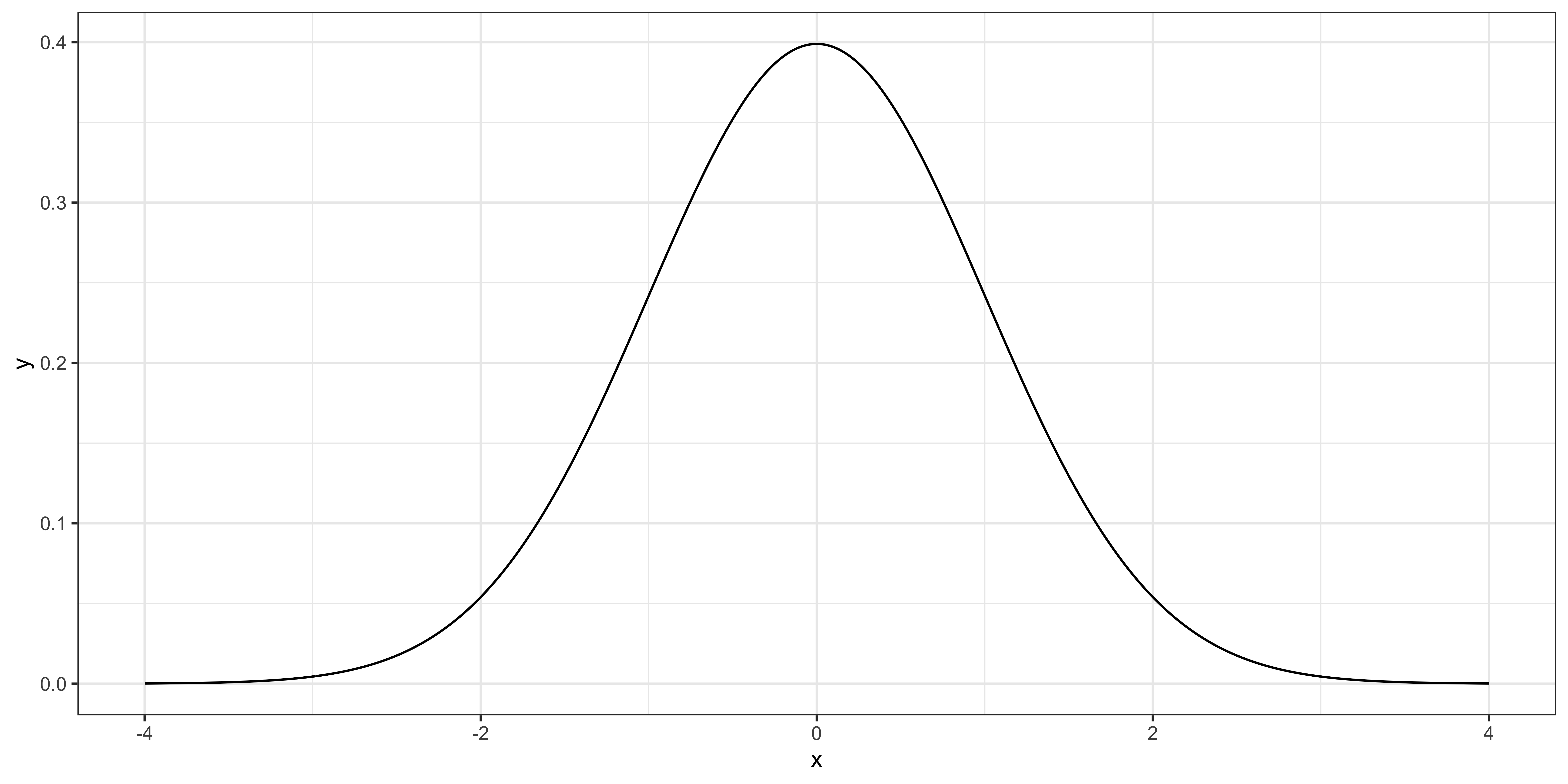
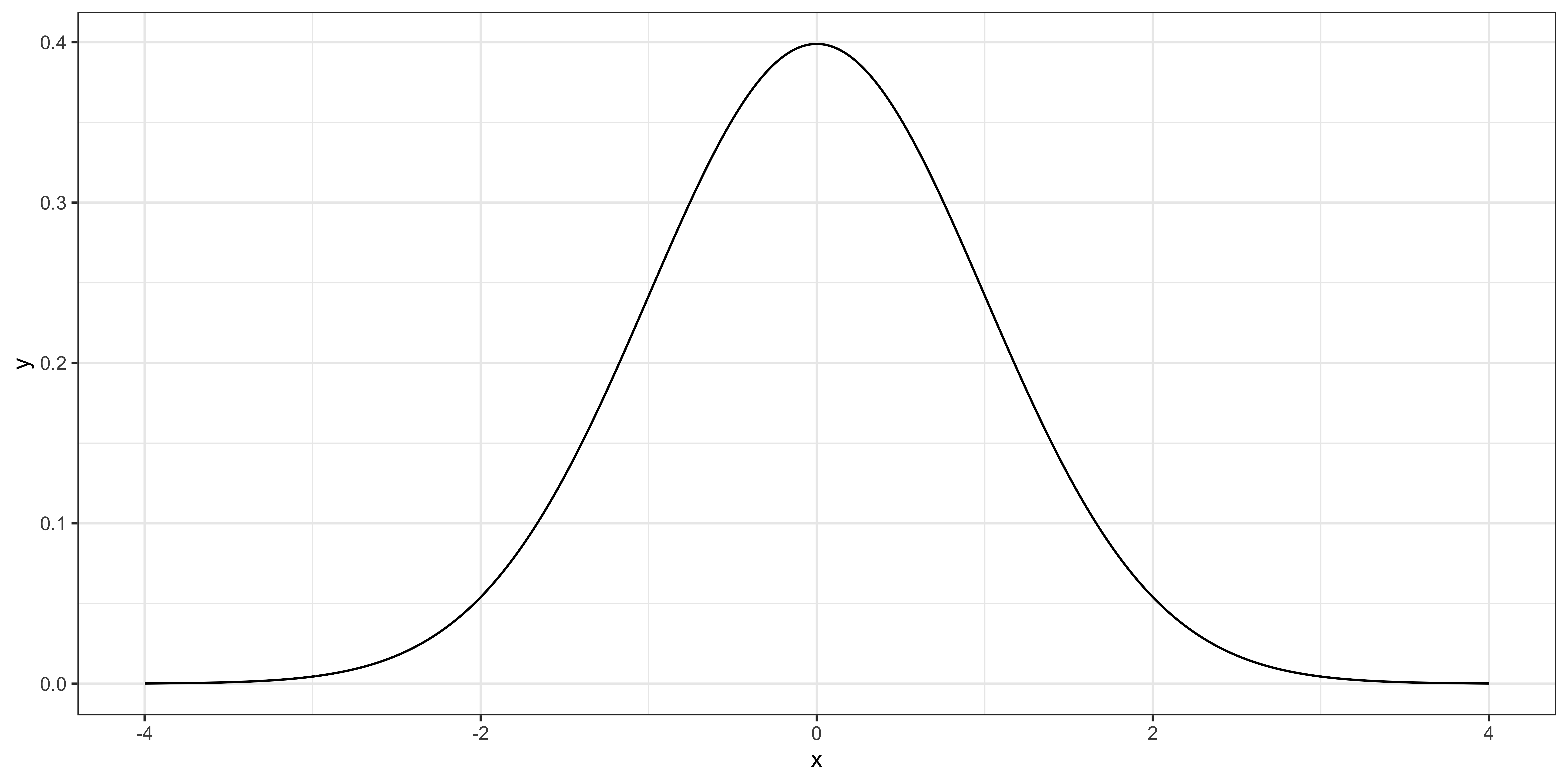
Now look at the figure in the right column. The horizontal axis contains possible values of this standardized statistic, and the vertical height is the standard Normal density. The curve is centered at zero and symmetric. Values near zero are common under H zero, while values far into either tail are rare. Because the goal was to test whether alpha is one “or not,” large positive and large negative values would both count as evidence. The curve is not the distribution of the raw x values or of theta itself. It is the distribution of the transformed statistic, conditional on the null being true. The next two tabs put actual sample means into this formula.
We established that \frac{\sqrt{J}}{2} \cdot (\theta - \alpha)\sim N(0, 1).
The null hypothesis is \alpha = 1.
If \alpha = 1 is indeed true, then \sqrt{J} \times (\theta - 1)/2 \sim N(0, 1).
In other words, if you take the sample mean, subtract the value under the null, multiply by the square root of the number of observations, and divide by 2, the result follows the standard Normal distribution like below.
Transcript
Now substitute the numbers from Case 1. The sample contains J equals one hundred observations, and its sample mean theta is two. Under H zero, the comparison value is one. Root one hundred is ten, the difference two minus one is one, and dividing ten times one by two gives a test statistic of five. In other words, the observed sample mean is five standard errors above the mean asserted by the null, because the standard error here is two over root one hundred, or zero point two.
Look at the standard Normal curve in the right column. Its horizontal axis shows possible values of the test statistic and its vertical height shows density. The displayed range ends around four, so a value of five is not even visible. It lies extremely far into the positive tail. Under a standard Normal distribution, an observation five standard deviations from zero is extraordinarily rare. For this two-sided question, we would count an equally extreme negative result as well.
The logic is a comparison between two explanations. One possibility is that alpha truly equals one and our sample happened to produce an extraordinarily unusual statistic. The other is that alpha does not equal one, so centering the statistic at one was inappropriate and the extreme value reflects a false null. Hypothesis testing controls how unusual a result must be before we choose the second interpretation and reject. This case clearly provides strong evidence against H zero, but we have not yet established a formal cutoff.
Suppose you have obtained 100 samples (J = 100) and calculated \theta (sample mean), which turned out to be 2.
Then, your test statistic is \sqrt{100} \times (2-1)/2 = 5.
How unlikely is it to get the number you got (5) if the null hypothesis is indeed true?
Transcript
Case 2 uses exactly the same statistic and null distribution, but different data. Here J is four hundred and the sample mean theta is one point zero two. Root four hundred is twenty. The sample mean exceeds the null value by only zero point zero two. Multiply twenty by zero point zero two and divide by two, and the test statistic is zero point two. Equivalently, the sample mean’s standard error is two over root four hundred, or zero point one, so the observed mean lies zero point two standard errors above one.
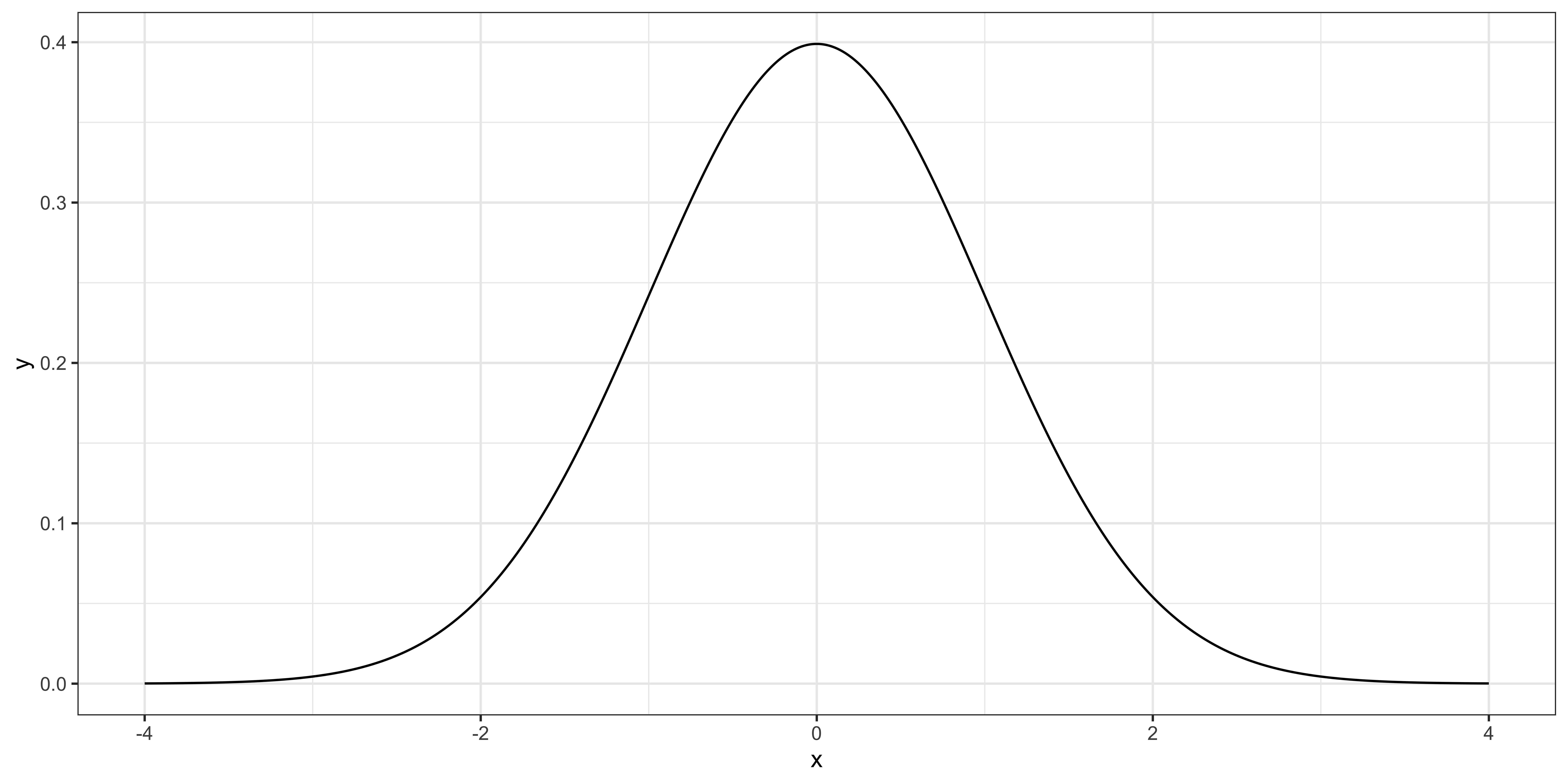
Find zero point two on the horizontal axis of the standard Normal curve. It sits very close to zero, in the high, central part of the density. Values around zero point two, and values even farther from zero, occur routinely when the null is true. This sample therefore gives us no compelling reason to doubt alpha equals one. The correct conclusion is to fail to reject the null, not to prove or accept it. A different sample could lead to a different estimate and decision.
Compare this tab with Case 1. The sample here is four times as large, which cuts the standard error in half, but the raw discrepancy from the null is only zero point zero two rather than one. A larger sample makes a given raw gap more statistically noticeable, yet it cannot manufacture evidence when the observed gap is tiny. The test statistic combines both ingredients: the size of the estimate’s departure from the null and the precision with which that departure was estimated.
Suppose you have obtained 400 samples (J = 400) and calculated \theta (sample mean), which turned out to be 1.02.
Then, your test statistic is \sqrt{400} \times (1.02-1)/2 = 0.2.
How unlikely is it to get the number you got (0.2) if the null hypothesis is indeed true?
Transcript
This aside explains why we standardize even though standardization is not logically required. In the left column, the alternative statistic is simply theta minus alpha, the sample mean’s raw estimation error. Because theta follows Normal with mean alpha and variance four over J, subtracting alpha gives a Normal distribution with mean zero and variance four over J. That is a perfectly valid null reference distribution. The complication is that it changes with J.
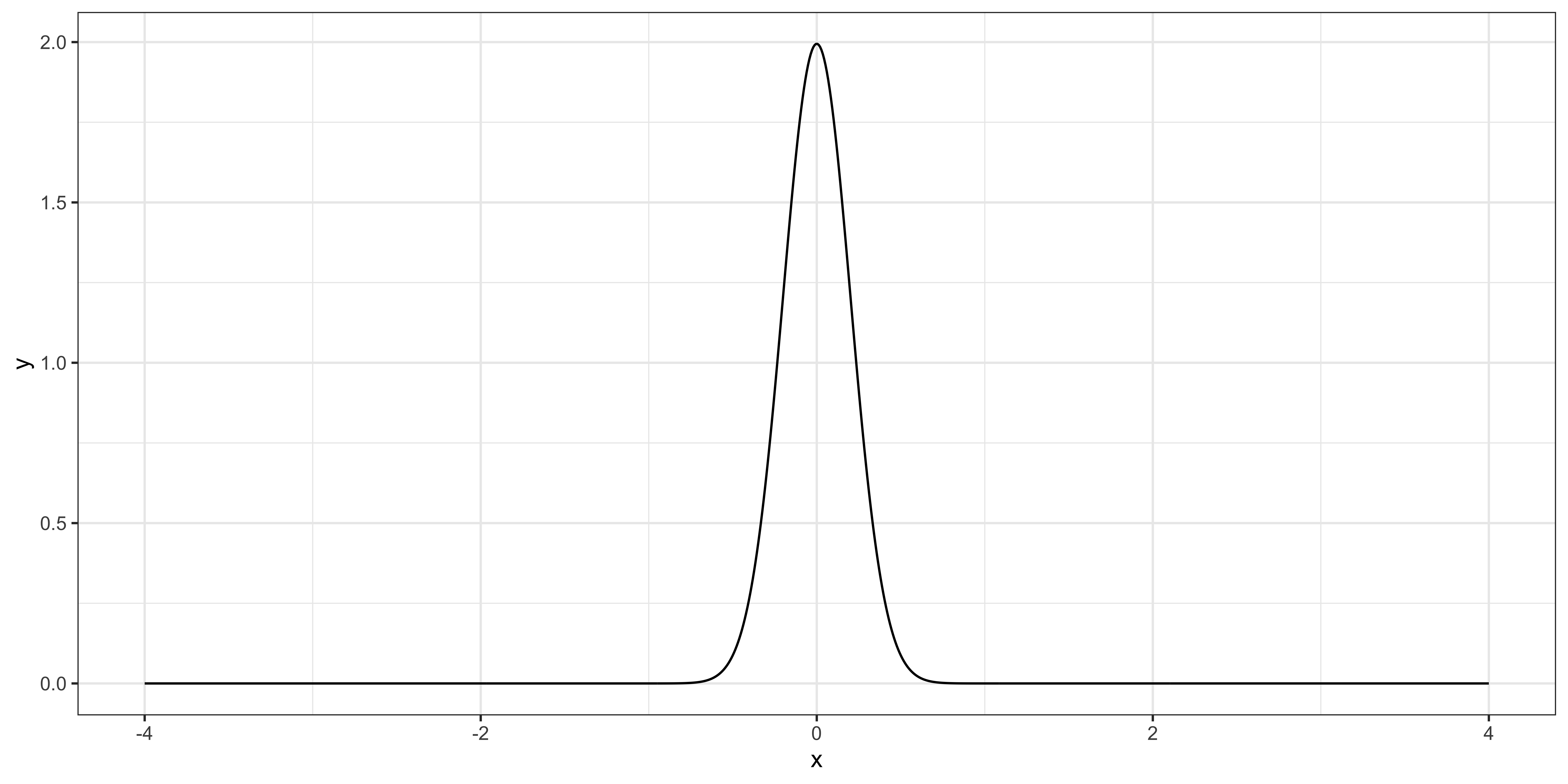
The figure on the right uses J equals one hundred. The horizontal axis is the raw difference theta minus alpha, and the vertical height is the density of a Normal distribution centered at zero with variance four over one hundred, which is zero point zero four, and standard deviation zero point two. That is why the curve is much narrower and taller than the standard Normal curve. Most raw differences should fall close to zero when the null is true.
Now reconsider Case 1 below the figure. Theta was two and the null value of alpha was one, so the raw statistic is two minus one, or one. On this distribution, one is five standard deviations above zero because one divided by zero point two equals five. That is exactly the standardized statistic we calculated before. The conclusion cannot depend on whether we measure the gap in original units or standard-error units, as long as we compare it with the matching distribution.
The callout gives the practical reason for normalization. Root J times theta minus alpha, divided by two, always follows the same standard Normal distribution, regardless of sample size. The unnormalized theta minus alpha requires a different variance, four over J, for every J. Standardization lets you reuse one reference distribution and its quantiles.
Note that you do not really need to use \sqrt{J} \times (\theta - \alpha)/2 as your test statistic.
You could alternatively use \theta - \alpha. But, in that case, you need to be looking at N(0, 4/J) instead of N(0, 1) to see how unlikely you get the number you got.
For example, when the number of observations is 100 (J = 100), the distribution of \theta-\alpha looks like the figure on the right.
Reconsider the case 1
Suppose you have obtained 100 samples (J = 100) and calculated \theta (sample mean), which turned out to be 2.
Then, your test statistic is 2-1 = 1.
Is it unlikely for you to get 1 if the null hypothesis is true?
The conclusion would be exactly the same as using \sqrt{J} \times (\theta - \alpha)/2 because the distribution under the null is adjusted according to the test statistic you use.
Transcript
This summary separates what a hypothesis test requires from what we usually do to meet that requirement. First, we need a test statistic whose probability distribution is known when the null hypothesis is true. A test statistic is a random quantity before the sample is drawn and a number after we insert our data. The null distribution tells us which realized numbers are ordinary and which are unusual under H zero. The examples listed here, a t distribution and a Normal distribution, are reference distributions we can use to assign tail probabilities or find critical values.
Second, we often have to transform the raw random variable we care about. In the example, the raw object was theta, the sample mean. Its distribution depended on the unknown alpha and on the sample size. We centered it by subtracting the null value and scaled it by its standard error. Under H zero, that transformed statistic followed the standard Normal distribution.
Once the statistic has a known null distribution, compute its realized value and ask whether a draw at least that extreme is plausible under H zero. The parenthetical note in the last bullet identifies the missing piece. We have not formally defined how small a probability must be before we reject.
What do we need?
- test-statistic of which we know the distribution (e.g., t-distribution, Normal distribution) assuming the null hypothesis
What do we (often) do?
- transform (most of the time) a raw random variable (e.g., sample mean in the example above) into a test statistic of which we know the distribution assuming that the null hypothesis is true
- e.g., we transformed the sample mean so that it follows the standard Normal distribution.
- check if the actual number you got from the test statistic is likely to happen or not (formal criteria has not been discussed yet)
Transcript
Your turn. This exercise has the same structure as the worked example, but the numbers change. Let x denote the annual-salary difference between graduates of University A and University B. The population model says x follows a Normal distribution with unknown mean alpha and known variance sixteen, so its population standard deviation is four. The substantive question is whether the average salary difference is ten, which makes the null H zero: alpha equals ten. Because the wording asks whether it is ten rather than whether it is greater or smaller, treat departures on either side as relevant.
For part two, let theta be the sample mean of four hundred independent observations. Its mean is alpha and its variance is the individual variance divided by the sample size: sixteen over four hundred, not sixteen. Its standard deviation, or standard error, is root sixteen over four hundred, which is four over root four hundred, or zero point two.
For part three, turn the sample mean into standard-error units. Subtract alpha and divide by four over root four hundred. That is the same as multiplying theta minus alpha by root four hundred over four. Under the Normal model, the result follows a standard Normal distribution. Under the null, replace alpha with ten so the statistic is computable.
Part four gives an observed sample mean of ten point two. Convert that to the standardized statistic, then use pnorm to find an upper-tail probability. As the prompt notes, pnorm of a value returns the probability that a standard Normal draw falls below that value, so an upper tail is one minus that number. Be precise about the question: it asks for the probability of observing a number greater than ten point two, not the two-sided probability of being at least zero point two away from ten. Try all four parts before opening the Answer tab. Finally, read the callout. In real work, the variance is not magically known, and we still need a formal rule for rejecting or failing to reject.
You have collected data on annual salary for those who graduated from University A and B. You are interested in testing whether the difference in annual salary between the universities (call it x) is 10 on average. You know (for unknown reasons) that the difference is distributed as N(\alpha, 16).
- What is the null hypothesis?
- Under the null hypothesis, what is the distribution of the sample mean when the number of observation is 400?
- Normalize the test statistic so that the transformed version follows N(0, 1).
- The actual difference you observed is 10.2. What is the probability that you observe a number greater than 10.2 if the null hypothesis is true? Use
pnorm(), which gives the probability that a standard Normal draw is below the value you hand it.
Transcript
Check each line against your solution. Line one states the null hypothesis: alpha equals ten. An alternative is not printed in the answer, but the original goal of testing whether the average is ten would normally pair it with alpha not equal to ten.
Line two gives theta’s sampling distribution as Normal with mean alpha and variance sixteen over four hundred. The variance comes from adding the variances of four hundred independent observations and then scaling their sum by one over four hundred. Numerically, sixteen over four hundred is zero point zero four, so the standard error is its square root, zero point two.
Line three standardizes theta. Read root four hundred over sixteen, times theta minus alpha. Root of the fraction is root four hundred divided by root sixteen, which is twenty divided by four, or five. That multiplier is the reciprocal of the standard error. After centering and scaling, the statistic follows the standard Normal distribution. Under H zero, alpha is replaced by ten.
Line four inserts the observed sample mean ten point two. Five times ten point two minus ten equals five times zero point two, which is one. The code cell calculates one minus pnorm of one. pnorm(1) is the standard Normal probability to the left of one, so subtracting from one gives the probability to the right. Running it returns about zero point one five nine, or fifteen point nine percent. Thus, if alpha truly equals ten, a sample mean greater than ten point two occurs about sixteen percent of the time. That is roughly one sample in six, so the upper-tail result is not unusual. The exercise explicitly asked only for the probability above ten point two, which is why the displayed code uses one tail.
- \alpha = 10
- \theta \sim N(\alpha, 16/400)
- \sqrt{\frac{400}{16}}\cdot (\theta - \alpha)
- The test statistic is 5 \times (10.2 - 10) = 1
Details of hypothesis testing on \beta_j
- Null and alternative hypothesis
- Significance level and power
- One-sided test
- Two-sided test
- One-sided vs two-sided
- p-value
- Example
Transcript
The courtroom analogy is useful because it makes the asymmetry between the two hypotheses explicit. Imagine that you are an attorney arguing that a defendant committed a crime. The null hypothesis corresponds to “the defendant is not guilty,” the position that remains unless the evidence crosses a prespecified threshold. The alternative corresponds to “the defendant is guilty,” the claim for which you are presenting evidence.
In a statistical application, the null is often a benchmark such as beta j equals zero, meaning no partial effect. The alternative states what would contradict that benchmark, such as beta j not equal to zero or beta j greater than zero. We compute how compatible the observed evidence is with the null. If the evidence would be sufficiently rare under H zero, we reject H zero in favor of H one.
Notice what the procedure does not say. A court that does not convict has not proved innocence; it has concluded that the evidence did not satisfy the burden of proof. Likewise, a statistical test that does not reject H zero has not proved the null. The proper phrase is “fail to reject,” not “accept.”
Statistical hypothesis testing involves two hypotheses: Null and Alternative hypotheses.
Pretend that you are an attorney who indicted a defendant who you think committed a crime.
Null Hypothesis
Hypothesis that you would like to reject (defendant is not guilty)
Alternative Hypothesis
Hypothesis you are in support of (defendant is guilty)
Transcript
The significance level formalizes how unlikely a result must be before we reject. The definition callout says it is the probability of rejecting H zero when H zero is actually true. That is a Type I error, analogous to convicting an innocent defendant. If you choose a five percent level and repeatedly apply the procedure in situations where the null is true, the procedure is designed to reject about five percent of the time in the long run.
A lower level requires stronger evidence. Moving from five percent to one percent means a test statistic has to be more extreme before we reject, so a true H zero is rejected less often. This reduces the long-run Type I error rate. It does not mean there is a one or five percent probability that the null is true. Frequentist significance treats the parameter and hypothesis as fixed and describes the behavior of the testing procedure across hypothetical repeated samples.
A lower significance level requires stronger evidence before rejecting the null and reduces the long-run probability of a Type I error. It does not tell us the probability that the null hypothesis is true.
Transcript
Now read the table by rows and columns. If H zero is true and you reject it, you make a Type I error. If it is true and you do not reject it, the decision is correct. If H zero is false and you reject it, the decision is correct. If it is false and you do not reject it, you make a Type II error.
The two bullets under the table explain the trade-off. The first says the significance level is a choice about how much Type I error you are willing to tolerate. The second says what that choice costs. Holding the design and sample size fixed, lowering the significance level makes rejection harder, which lowers Type I error but increases Type II error: there are more cases where H zero is false and you still fail to reject it.
There are two ways to be wrong, and they trade off against each other:
| H_0 is true | H_0 is false | |
|---|---|---|
| You reject H_0 | Type I error (probability = significance level) | correct |
| You do not reject H_0 | correct | Type II error |
- the significance level is a choice about how much Type I error you will tolerate
- pushing it down from 5% to 1% requires stronger evidence, so you reject less often. That means more Type II error: cases where H_0 is false but you fail to reject it
Transcript
One minus the probability of Type II error is called power. It is the probability that the test rejects H zero when H zero is false. Power is not a single number for a test; it depends on how far the true beta j is from the value stated in H zero. When the true value is close to the null value, the test rarely rejects; when it is far away, the test rejects most of the time. The One-sided vs two-sided tab, after the two tests, draws power as an area for one particular true value of beta j.
This is why not rejecting H zero does not mean H zero is true. The most common null is beta j equals zero, and in that case the same point reads: “not statistically significant” does not mean “no effect.” It may mean that the test had too little power to tell the true beta j apart from zero given the sampling noise. The same reasoning applies to any other null value, such as beta j equals one.
- 1 - P(\text{Type II error}) is called the power of the test: the probability of rejecting H_0 when it is false (drawn in the One-sided vs two-sided tab). It depends on how far the true \beta_j is from the value in H_0
- this is why “not rejecting H_0” does not mean “H_0 is true”. For the common case H_0: \beta_j = 0, “not statistically significant” does not mean “no effect”. It may just mean your test had too little power to detect the difference
Transcript
This tab states the hypotheses of a one-sided test. H zero says beta j equals zero. H one says beta j is greater than zero. The alternative is directional: it claims not just that beta j differs from zero, but that it differs in one particular direction.
That direction decides which t-statistics count as evidence against H zero. Under H one, beta j hat tends to come out above zero, so the t-statistic tends to be large and positive. Only a t-statistic far above zero therefore supports H one, and the rejection region sits in the upper tail of the t distribution only. A large negative t-statistic does not count as evidence for H one, even though it is far from zero, because it points in the direction opposite to the one H one claims.
If the alternative were instead beta j less than zero, everything flips: only a t-statistic far below zero counts, and the rejection region sits in the lower tail. The next tab draws the upper-tail rule at the five percent level, and the One-sided vs two-sided tab, after the two-sided test, shows why placing all of the significance level in one tail is worth doing when H one is one-sided.
H_0: \beta_j = 0
H_1: \beta_j > 0
- only a t-statistic far above 0 counts as evidence for H_1
- so the rejection region is in the upper tail of the t-distribution only
- (for H_1: \beta_j < 0, it is the lower tail instead)
Transcript
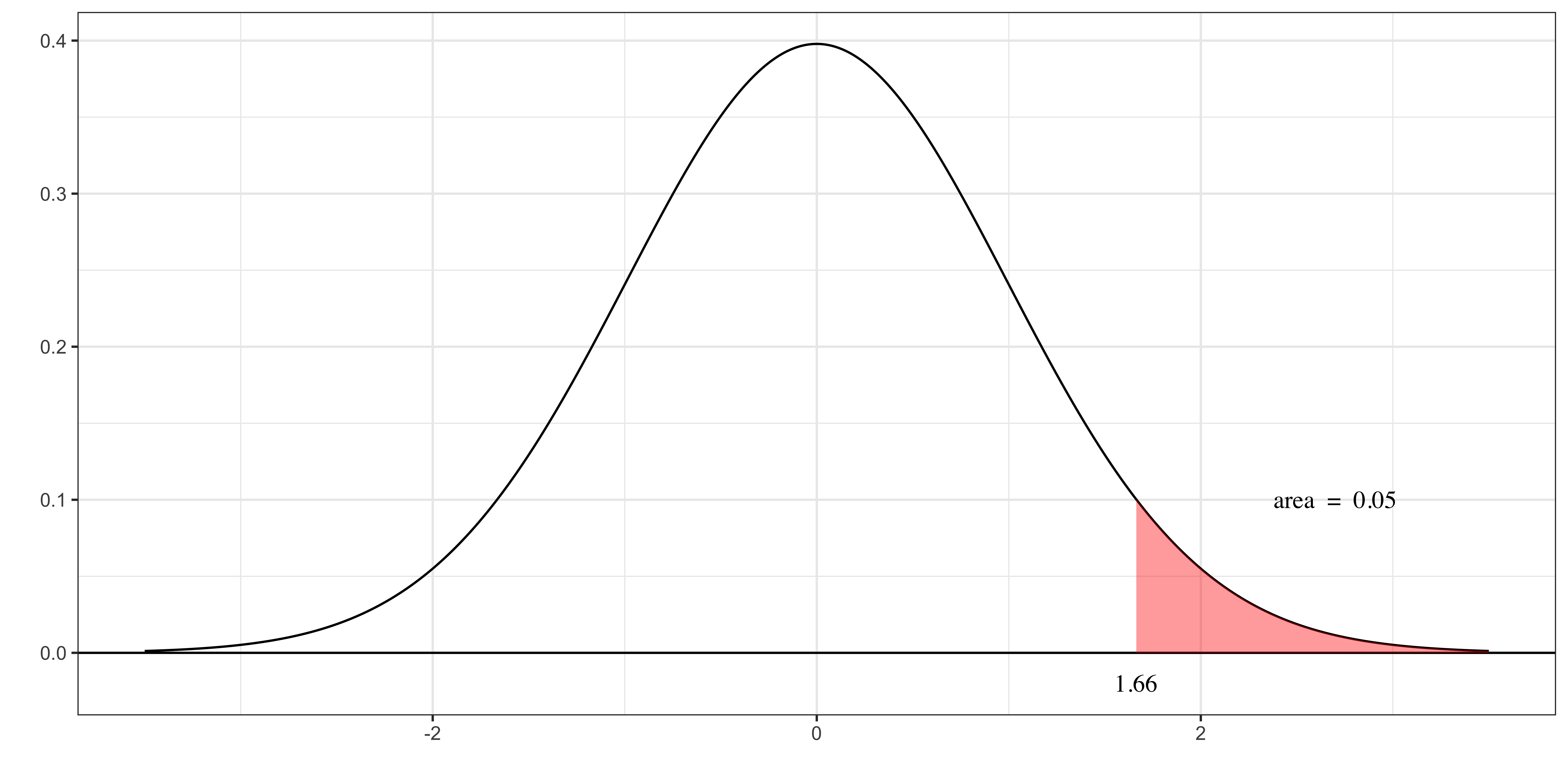
This picture implements the one-sided upper-tail test from the previous tab, H zero: beta j equals zero against H one: beta j greater than zero, at the five percent significance level. The title above the figure says what the curve is: the distribution of the t-statistic if H zero is true. The t-statistic is beta j hat minus beta j, divided by its estimated standard error. Under the null beta j equals zero, so the numerator becomes beta j hat and, under the classical assumptions, the statistic follows this t distribution with five hundred and twenty-two residual degrees of freedom.
On the figure, the horizontal axis contains possible t-statistics and the vertical height is the t density. The curve is centered at zero and symmetric, although this test uses only its positive tail because H one is beta j greater than zero. The red area is the upper five percent of the total area under the curve. Its left edge, marked by the red vertical line, is about one point six five for this many degrees of freedom: the ninety-fifth percentile of the t distribution.
The two red labels on the figure name the two numbers, and it is worth keeping them distinct. The label at the top of the vertical line says “critical value equals one point six five”. That is a value on the t-statistic scale, a point on the horizontal axis. The label with the arrow pointing into the red area says “significance level equals five percent”. That is a probability, the size of the red area, and it is chosen before the test. The critical value follows from that choice together with the degrees of freedom; with different degrees of freedom, the same five percent level produces a different critical value.
The Decision Rule box in the left column says to reject H zero if the observed t-statistic is greater than the critical value. The sentence under it says what the five percent means. If H zero is true, only five percent of repeated samples generate a statistic in the red area, so the rule rejects a true H zero in five percent of samples. That is the Type I error probability. Be careful with the direction of this statement. It is the probability of rejecting given that H zero is true. It is not the probability that H zero is true given that you rejected, and it is not “a five percent chance that you are wrong” after a particular rejection. A statistic in the red area can still occur under a true null, so rejection is not certainty; it means the result crossed the evidence threshold we chose.
If H_0 is true, this rule rejects it in 5% of samples (Type I error).
Transcript
This tab states the hypotheses of a two-sided test. H zero again says beta j equals zero. H one says beta j is not equal to zero. Unlike the one-sided alternative, this one does not commit to a direction: beta j could be above zero or below zero.
So departures from zero in either direction count as evidence against H zero. A t-statistic far above zero indicates an estimate above zero, and a t-statistic far below zero indicates one below zero; both are unlikely if H zero is true, and both are what H one allows. The rejection region therefore occupies both tails of the t distribution, and the significance level is split between them. The next tab draws that rule at the five percent level, and the One-sided vs two-sided tab shows why both tails are needed when H one is two-sided.
H_0: \beta_j = 0
H_1: \beta_j \ne 0
- a t-statistic far from 0 in either direction counts as evidence for H_1
- so the rejection region is in both tails, with the significance level split between them
Transcript
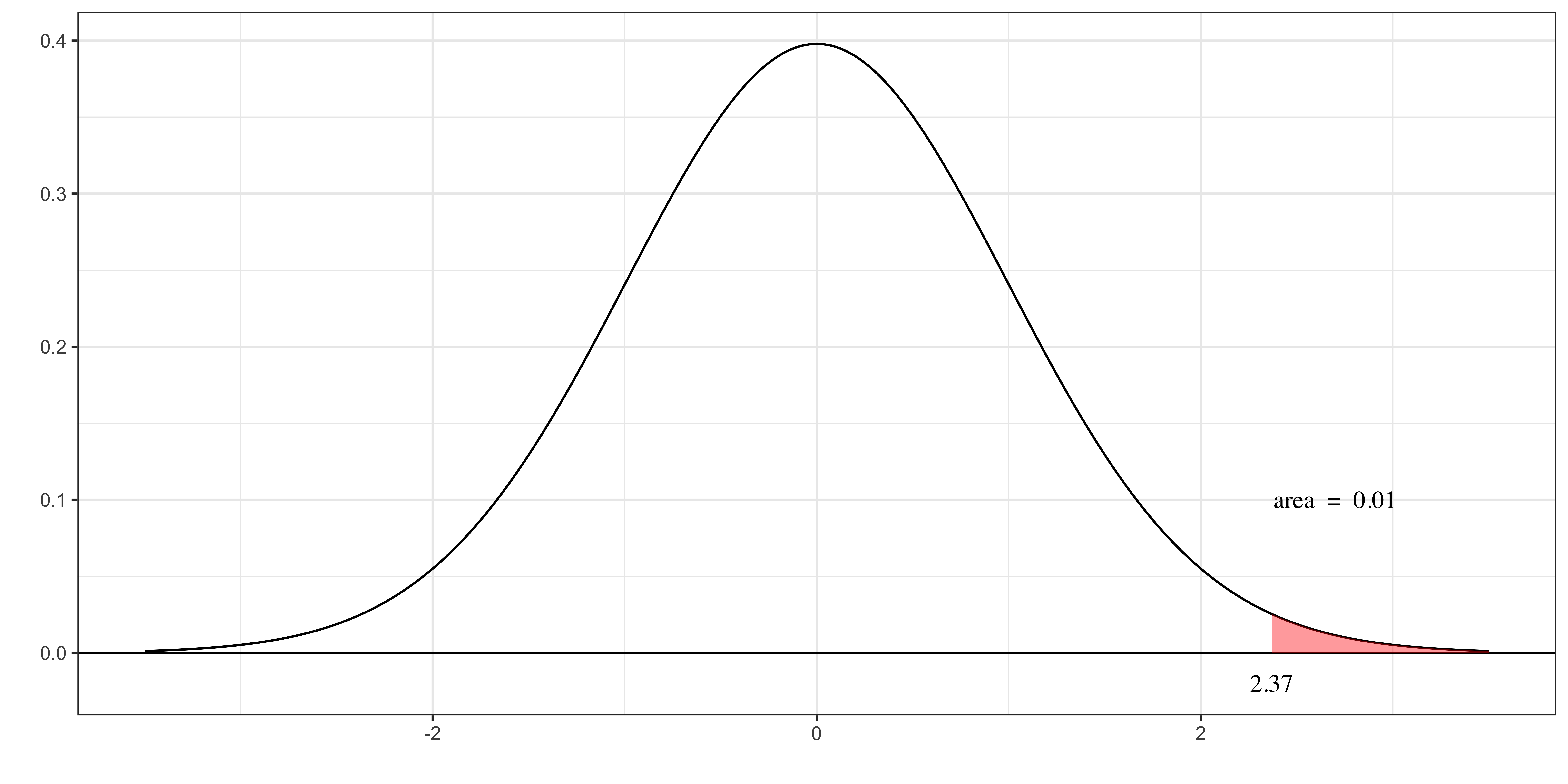
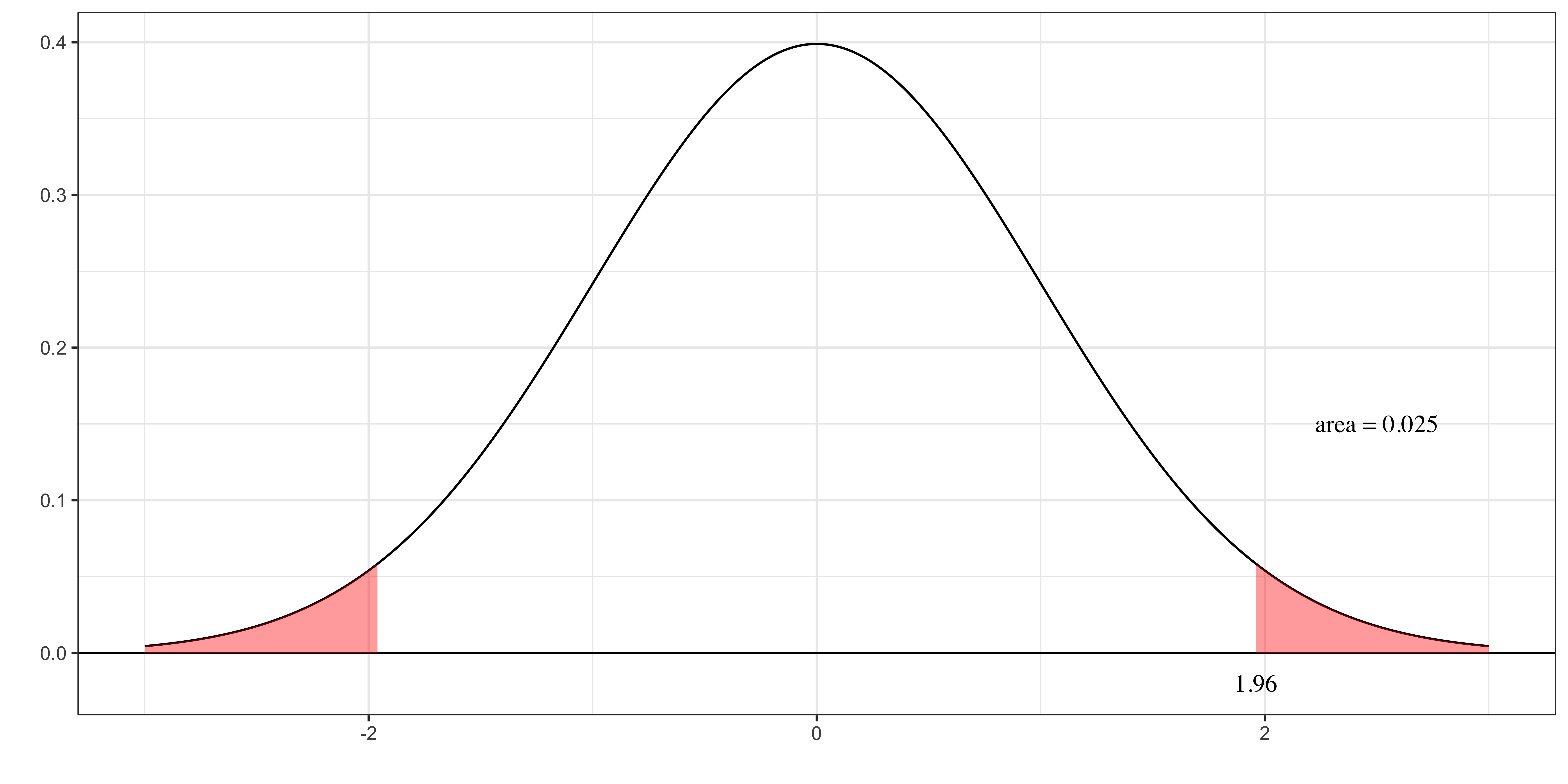
This picture implements the two-sided test from the previous tab, H zero: beta j equals zero against H one: beta j not equal to zero, at the five percent significance level. Both positive and negative departures from zero now count against H zero. The title above the figure says what the curve is: the distribution of the t-statistic if H zero is true. It is the same t distribution with five hundred and twenty-two degrees of freedom as in the one-sided Decision rule tab, because the statistic and its null distribution have not changed. The alternative changes the rejection region, not the statistic’s null distribution.
The total significance level is still five percent. Because evidence in either direction matters, split that probability evenly: two point five percent in the left tail and two point five percent in the right tail. The positive boundary is the ninety-seven point five percentile of the t distribution, about one point nine six, and symmetry puts the negative boundary at about minus one point nine six. Those are farther from zero in absolute value than the one-sided five percent boundary because each tail receives less area.
Look at the figure. The horizontal axis is the t-statistic, the vertical height is density, and both extreme ends are shaded red. The unshaded center contains ninety-five percent of the null distribution. There are now two red vertical lines, each labelled at the top with its critical value: minus one point nine six on the left and one point nine six on the right. The label in the middle, “significance level equals five percent, two point five percent in each tail”, has two arrows, one pointing into each red area, because the significance level is the two areas added together.
The Decision Rule box in the left column expresses both boundaries compactly: reject if the absolute value of the observed t-statistic is greater than about one point nine six. Taking the absolute value treats equally strong positive and negative evidence the same way. The sentence under it gives the Type I error probability: if H zero is true, the statistic lands in one of the two red areas in five percent of samples, so the rule rejects a true H zero in five percent of samples. Do not halve the critical value or compare a signed statistic only with the positive boundary without taking its absolute value.
If H_0 is true, this rule rejects it in 5% of samples (Type I error).
Transcript
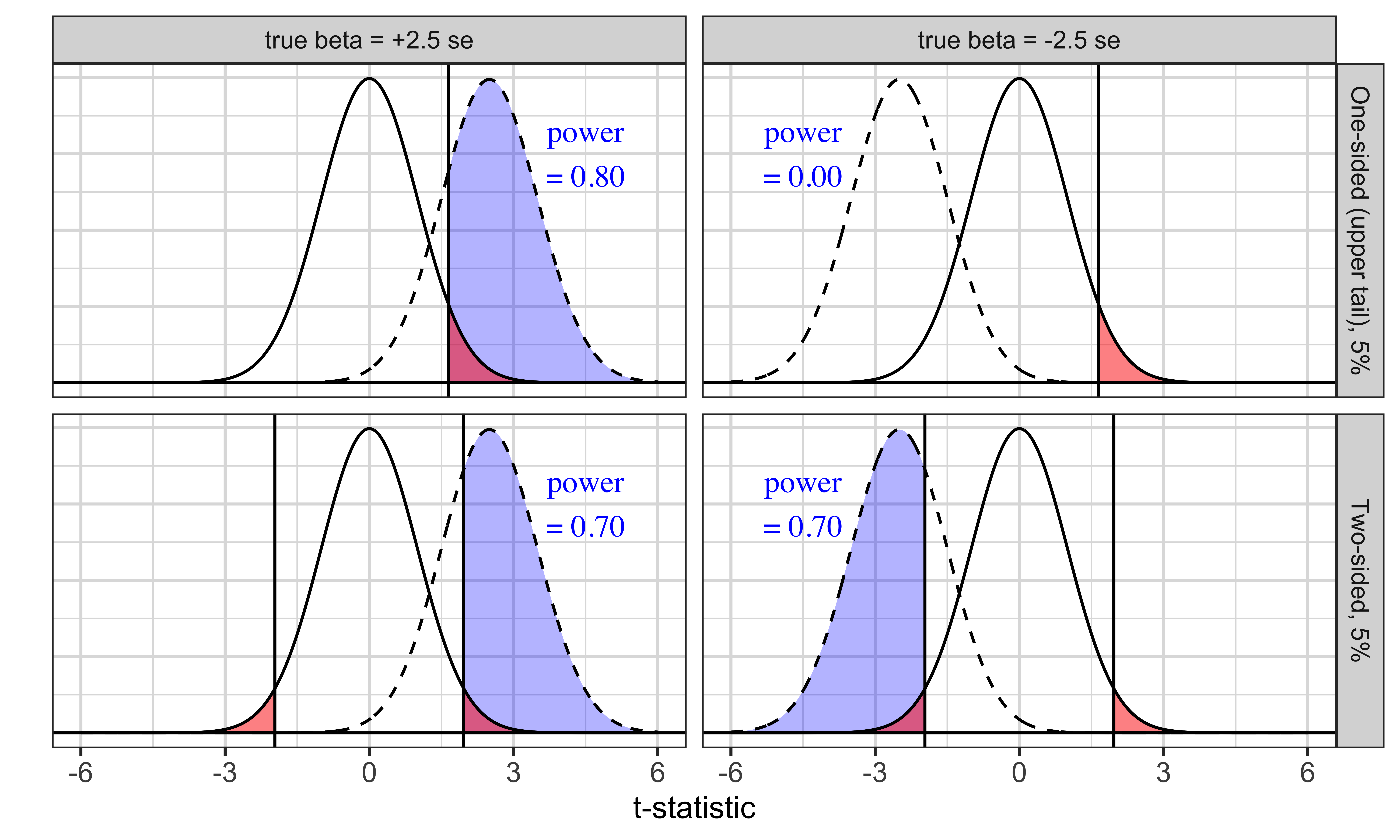
This tab and the next answer why the alternative decides where the rejection region goes, using power. This tab takes the one-sided alternative, H one: beta j greater than zero. Why put the whole significance level in the upper tail? Suppose H one is true and the true beta j is two point five times the standard error of beta j hat, above zero. The figure has two panels for that same truth. The top panel is the one-sided upper-tail test at the five percent level; the bottom panel is the two-sided test at the five percent level. In each panel, the solid curve is the distribution of the t-statistic if H zero were true, the dashed curve is its actual distribution under the true beta j, the vertical lines are the critical values, the red area is the Type I error probability, and the blue area, the part of the dashed curve beyond a critical value, is the power, printed in blue.
Both tests reject a true H zero five percent of the time: the red areas add up to five percent in both panels. The difference is where that five percent is placed. The one-sided test puts all of it in the upper tail, so its critical value is only about one point six five, and about eighty percent of the dashed curve lies beyond it. Its power is about zero point eight zero.
The two-sided test puts two point five percent in each tail. The lower-tail region is wasted here: a t-statistic centred near two point five essentially never lands below minus one point nine six, so the blue area on the left is too small to see. And because the upper tail now gets only two point five percent, the upper critical value moves out to about one point nine six, which cuts off more of the dashed curve. The two-sided test’s power is about zero point seven zero.
So when beta j can only be above zero, as H one says, the one-sided test detects a true effect more often than the two-sided test at the same significance level. That is the reason to run a one-sided test. The next tab shows the other side of this trade-off: what happens when H one is two-sided and beta j might be below zero.
- suppose the true \beta_j is 2.5 \times\, se(\widehat{\beta}_j), above 0 as H_1 says
- both tests reject a true H_0 5% of the time (red)
- one-sided puts all 5% in the upper tail: critical value 1.65, power 0.80
- two-sided spends half of it in the lower tail, where the true distribution almost never lands: the upper critical value moves to 1.96 and power falls to 0.70
Transcript
The previous tab showed that, when the true beta j is above zero, a one-sided test pointed upward has more power than a two-sided test at the same significance level. This tab shows what the two-sided test buys in exchange, when H one is beta j not equal to zero. The null is again H zero, beta j equals zero, and both tests reject a true null five percent of the time. The one-sided test puts all of that five percent in the upper tail, with a critical value of about one point six five. The two-sided test splits it, two point five percent in each tail, with critical values of about minus one point nine six and one point nine six.
The figure is a grid of four panels. The rows are the two tests: the one-sided upper-tail test on top, the two-sided test below. The columns are two possible truths. In the left column the true beta j is two point five standard errors above zero; in the right column it is two point five standard errors below zero. In every panel the solid curve is the distribution of the t-statistic if H zero were true, with the Type I error area shaded red, and the dashed curve is its actual distribution under that column’s truth. The vertical lines are the critical values, and the blue area, the part of the dashed curve beyond a critical value, is the power, printed in blue in each panel.
Read the left column first. The truth is above zero, the dashed curve is centred near two point five, and the one-sided test has power of about zero point eight zero against about zero point seven zero for the two-sided test. This is the comparison from the previous tab: the one-sided test wins when the truth is on the side it points to.
Now read the right column. The truth is below zero, so the dashed curve is centred near minus two point five. The one-sided test only rejects when the t-statistic is above one point six five, and a t-statistic centred at minus two point five essentially never gets there. Its power is about zero point zero zero zero zero two, effectively zero: it will almost never detect this effect, no matter how real it is. The two-sided test has a rejection region on the left as well, and the dashed curve now falls mostly beyond minus one point nine six, so its power is again about zero point seven zero, exactly the same as in the left column, because the test treats both sides symmetrically.
So when H one is beta j not equal to zero, the true beta j could be on either side, and the question is which test does better across both possibilities. The one-sided test does slightly better on one side, zero point eight zero against zero point seven zero, and fails completely on the other side. The two-sided test gives up a little power on the side you might have guessed, in exchange for keeping the same power on the side you did not guess. That is why a two-sided alternative calls for rejection regions on both sides. A one-sided test is appropriate only when you have a good justification that beta j can never be on the other side, not merely that you expect it to be on one side. The justification has to come from outside the data, for example from economic theory or from how the variable is constructed, and it has to be strong enough that a value on the other side is ruled out, because the one-sided test has essentially no power to detect it if it happens.
The sign of beta j hat is not such a justification, and this is a real temptation in practice. Suppose the two-sided p-value is zero point zero eight and the estimate is positive. It is tempting to say that you expected a positive effect all along, switch to a one-sided test, and report half the p-value, zero point zero four. But choosing the side after seeing the estimate means you would have rejected in whichever tail the estimate happened to land. That puts a five percent rejection region in each tail, so a true H zero is rejected ten percent of the time, not the five percent you report.
- H_1: \beta_j \neq 0: the true \beta_j may be above or below 0. Both tests reject a true H_0 5% of the time
- true \beta_j above 0 (left): one-sided wins, 0.80 vs 0.70
- true \beta_j below 0 (right): the upper-tail test almost never rejects (power 0.00); two-sided still 0.70
- two-sided gives up a little power on one side to keep it on the other. Use one-sided only if you have a good justification (e.g. from theory) that \beta_j can never be on the other side. The sign of \widehat{\beta}_j is not such a justification
Transcript
The p-value packages the same tail comparison into a single number. The definition callout gives two equivalent readings. It is the smallest significance level at which the observed result would lead you to reject H zero. It is also, assuming H zero is true, the probability of drawing a test statistic at least as extreme as the one actually observed.
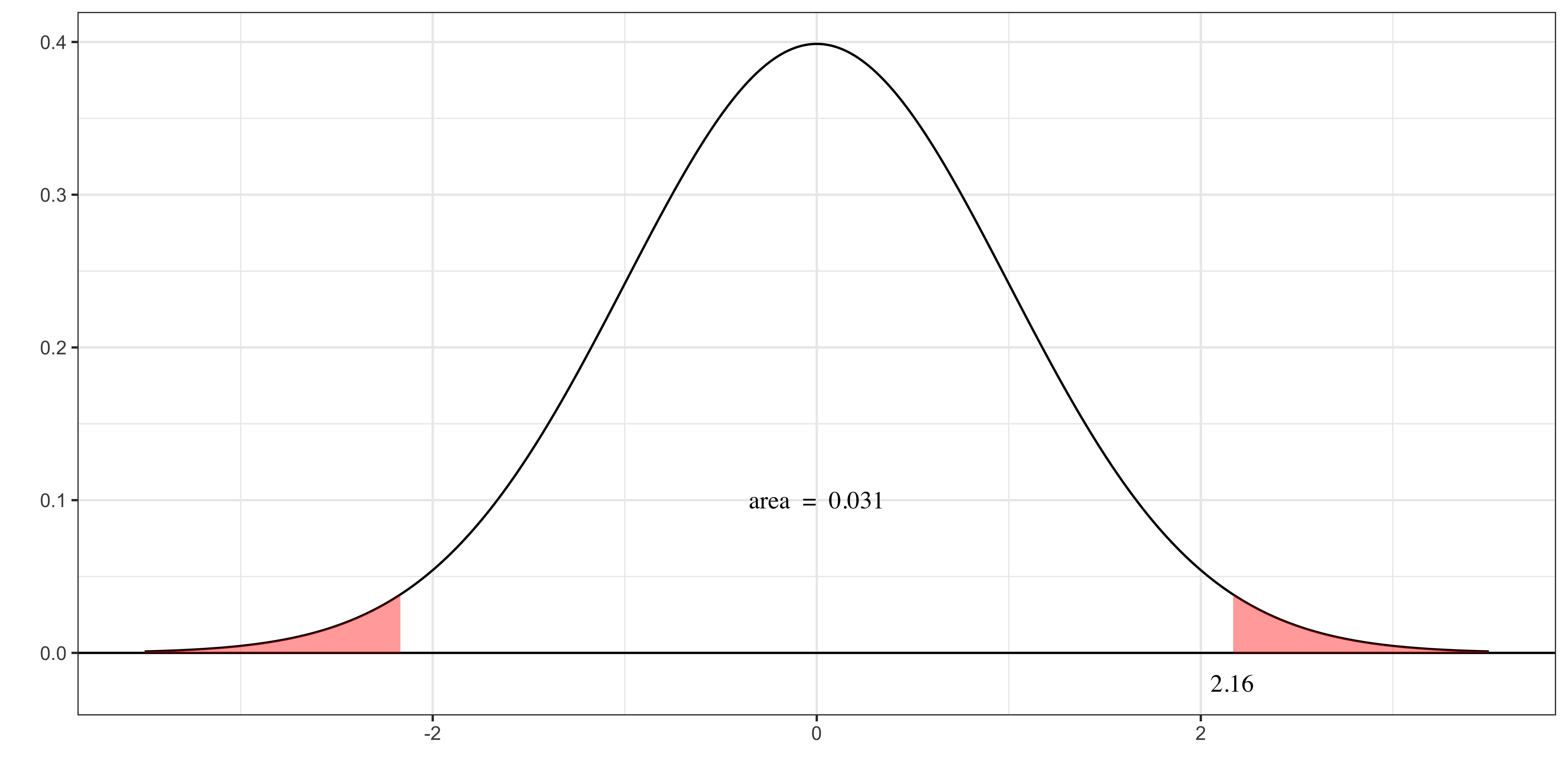
This slide uses a two-sided test: H zero, beta j equals zero, against H one, beta j not equal to zero, with an observed t-statistic of two point one six. The first bullet in the left column states the hypotheses and that result. On the figure, the horizontal axis is the t-statistic and the vertical height is the t density under H zero, the same t distribution with five hundred and twenty-two degrees of freedom used in the One-sided test and Two-sided test tabs. The red vertical line on the right, labelled “observed t equals two point one six”, marks the statistic we actually got. The red line on the left, at minus two point one six, is its mirror image. Both tails beyond those lines are shaded because, for a two-sided alternative, a statistic equally far from zero in either direction counts as at least as extreme.
The label in the middle, with an arrow into each red area, gives the combined shaded area: about zero point zero three one, or three point one percent, which is about zero point zero one five six in each tail. That combined area is the two-sided p-value, and the second bullet reads it in words: if H zero is true, a t-statistic at least this far from zero happens with probability zero point zero three one. Compare this figure with the figure in the Decision rule tab of the Two-sided test tab. There, we fixed the red area at five percent and read off the cutoff. Here we do the reverse: we put the cutoff at the statistic we observed and read off the red area.
That reversal is why the third bullet holds. If you selected a significance level of exactly three point one percent, the critical value would sit exactly at the observed statistic. At any larger level, such as five percent, the critical value is closer to zero, the observed statistic lies beyond it, and you reject. At any smaller level, such as one percent, the critical value lies farther out than two point one six and you fail to reject. So three point one percent is the smallest significance level at which you would reject.
The Decision rule box in the left column summarizes the comparison: reject when the p-value is below the chosen significance level. The sentence under it says this always agrees with comparing the t-statistic with the matching critical value, provided the same distribution, degrees of freedom, and sidedness are used.
- H_0: \beta_j = 0 vs H_1: \beta_j \neq 0 (two-sided); suppose the t-statistic you got is 2.16
- If H_0 is true, a t-statistic at least this far from 0 (either side) happens with probability 0.031 (the two red areas): this is the p-value
- So 3.1% is the smallest significance level at which you would reject H_0
This always gives the same result as comparing the t-statistic with the critical value.
Transcript
Work through this example from the model to the decision. The estimated log-wage equation includes education, experience, and tenure. The coefficient on experience is zero point zero zero four one.
The estimated standard error of the experience coefficient is zero point zero zero one seven. We test H zero: beta exper equals zero against the one-sided alternative beta exper greater than zero. Under H zero, the t-statistic is the estimate minus zero, divided by its estimated standard error. That gives zero point zero zero four one divided by zero point zero zero one seven, or about two point four one. The statistic says the estimate is about two point four one standard errors above the null value.
The model has n equals five hundred and twenty-six observations and k equals three explanatory variables, excluding the intercept. Residual degrees of freedom are therefore five hundred and twenty-six minus three minus one, or five hundred and twenty-two. Because the alternative is positive and the significance level is one percent, use an upper-tail critical value rather than splitting the probability across two tails. qt(0.99, 522) returns about two point three three, the ninety-ninth percentile of the appropriate t distribution.
Finally compare on the same scale. Two point four one is greater than two point three three, so the observed statistic lies in the one-percent upper-tail rejection region. We reject H zero in favor of a positive experience effect at the one percent level.
Estimated Model
The impact of experience on wage:
- log(wage) = 0.284+0.092\times educ+0.0041\times exper + 0.022 \times tenure
- \widehat{se(\widehat{\beta}_{exper})} = 0.0017
- n = 526
Hypothesis
- H_0: \beta_{exper}=0
- H_1: \beta_{exper}>0
Test
t-statistic = 0.0041/0.0017 = 2.41
The critical value is the 99% quantile of t_{526-3-1}, which is 2.33 (it can be obtained by qt(0.99, 522))
Since 2.41 > 2.33, we reject the null in favor of the alternative hypothesis at the 1% level.
Confidence Interval (CI)
Transcript
The definition callout gives the repeated-sampling meaning of a ninety-five percent confidence interval. Imagine repeatedly drawing new random samples using the same design and, for each sample, calculating an interval with the same formula. The endpoints change from sample to sample because the estimate and its standard error change. In the long run, ninety-five percent of those intervals will cover the fixed true parameter and five percent will miss it, provided the assumptions behind the procedure hold.
Confidence therefore describes the coverage rate of the interval-generating procedure. Before sampling, the endpoints are random and the procedure has a ninety-five percent probability of producing an interval that covers the parameter. Once a specific sample has been observed and its interval calculated, the endpoints are fixed. The population parameter is also fixed. That realized interval either contains the true parameter or it does not.
The lower half identifies the common incorrect interpretation: “there is a ninety-five percent probability that this particular realized interval includes the true parameter.” In the frequentist framework used here, that is not what the statement means. We do not assign a probability distribution to the fixed beta after seeing the data. The ninety-five percent refers to what the method would do over repeated samples.
What confidence interval is not
The probability that a realized CI calculated from specific sample data includes the true parameter
Transcript
This slide gives the general recipe for a confidence interval. Start with what a confidence interval is about: it is a range for an unknown population parameter, which we call theta. It is not a range for a statistic. The recipe has three steps.
Step one. Find a quantity that involves theta and the data, and whose probability distribution is completely known even though theta itself is unknown. The example on the slide is beta j hat minus beta j, divided by the estimated standard error of beta j hat. Under MLR one through MLR six, this quantity follows a t distribution with n minus k minus one degrees of freedom, and that distribution does not depend on the unknown beta j. Beta j hat alone would not work, because its distribution is centered on the unknown beta j, so we could not compute its quantiles.
Step two. Find the range that holds the middle A percent of that known distribution. The A percent in the middle leaves one hundred minus A percent outside, and we split that equally between the lower and upper tails. So the lower bound is the open parenthesis one hundred minus A close parenthesis, divided by two, percent quantile, and the upper bound is one hundred minus that same tail percentage. A quantile is the value with the stated proportion of the distribution at or below it. Pay attention to the parentheses. For A equals ninety-five, calculate one hundred minus ninety-five first, obtaining five, then divide by two to obtain two point five. Reading it as one hundred minus A divided by two would instead produce fifty-two point five, which is completely different. The upper percentile is one hundred minus two point five, or ninety-seven point five. Before the sample is drawn, the quantity from step one falls inside this range with probability A percent.
Step three. The statement “the quantity is inside this range” involves theta, so we can rewrite it as a statement about theta alone: theta lies between a lower value and an upper value, both computed from the data. That range for theta is the A percent confidence interval. Notice that the range from step two is not itself a confidence interval. It is a range of values of a quantity with a known distribution, and it contains that quantity with probability A percent. It becomes a confidence interval only after step three turns it into a range for the parameter.
A confidence interval is a range for an unknown parameter \theta.
- Find a quantity that involves \theta and the data, and whose distribution is known even though \theta is unknown. Example: \frac{\widehat{\beta}_j - \beta_j}{\widehat{se(\widehat{\beta}_j)}} \sim t_{n-k-1}.
- Find the range that holds the middle A\% of that distribution. Before the sample is drawn, the quantity falls in this range with probability A\%.
- lower bound: (100 - A)/2 percent quantile
- upper bound: 100-(100 - A)/2 percent quantile
- Rewrite “the quantity is inside this range” as a statement about \theta. The resulting range for \theta is the A\% confidence interval.
Transcript
This slide derives a confidence interval for beta j from the t-statistic. Under MLR one through MLR six, beta j hat minus beta j, divided by the estimated standard error of beta j hat, follows a t distribution with n minus k minus one degrees of freedom. Beta j hat is the sample coefficient estimate, beta j is the fixed population coefficient, the denominator is the estimated sampling standard deviation, n is the sample size, and k counts explanatory variables other than the intercept.
For an A percent central interval, define Q sub l as the open parenthesis one hundred minus A close parenthesis over two percentile of that t distribution. Define Q sub h as the one hundred minus open parenthesis one hundred minus A close parenthesis over two percentile. Because the t distribution is symmetric around zero, Q sub l is negative and Q sub h is the corresponding positive value.
Those quantiles initially bound the standardized statistic, but our target is beta j. Solve the displayed statistic for beta j. If t denotes a possible value of the standardized expression, multiply by the estimated standard error to get beta j hat minus beta j, then rearrange: beta j equals beta j hat minus t times the estimated standard error. The minus sign reverses which t quantile maps to which beta endpoint. Symmetry makes the familiar final result beta j hat plus a negative critical amount for the lower bound and beta j hat plus a positive critical amount for the upper bound.
That is what the final bullets state. Multiply Q sub l by the estimated standard error and add beta j hat for the lower bound. Multiply Q sub h by the same standard error and add beta j hat for the upper bound. Since Q sub l is negative and Q sub h positive, the interval is centered on beta j hat and extends the same number of standard errors in both directions. A larger standard error makes the interval wider, signaling less precision. The next tabs calculate a ninety-percent interval for the education coefficient.
Under the assumption of MLR.1 through MLR.6 (which includes the normality assumption of the error), we learned that
\frac{\widehat{\beta}_j - \beta_j}{\widehat{se(\widehat{\beta}_j)}} \sim t_{n-k-1}
So, following step 2 of the general procedure, the range that contains \frac{\widehat{\beta}_j - \beta_j}{\widehat{se(\widehat{\beta}_j)}} with probability A% is
- lower bound: (100 − A)/2% quantile of the t_{n-k-1} distribution (let’s call this Q_l)
- upper bound: 100 - (100 − A)/2% quantile of the t_{n-k-1} distribution (let’s call this Q_h)
But, we want the A% CI of \beta_j, not \frac{\widehat{\beta}_j - \beta_j}{\widehat{se(\widehat{\beta}_j)}}. Solving for \beta_j,
\beta_j = \widehat{\beta}_j - t_{n-k-1}\times \widehat{se(\widehat{\beta}_j)}
So, to get the A% CI of \beta_j (step 3), we scale the range [Q_l, Q_h] by \widehat{se(\widehat{\beta}_j)} and then shift by \widehat{\beta}_j. Because the t distribution is symmetric, the minus sign above just swaps which quantile lands on which end:
- lower bound: Q_l \times \widehat{se(\widehat{\beta}_j)} + \widehat{\beta}_j
- upper bound: Q_h \times \widehat{se(\widehat{\beta}_j)} + \widehat{\beta}_j
Note that Q_l is negative and Q_h is positive.
Transcript
This tab reconstructs the wage-level regression for the confidence-interval example. The first cell calls feols with wage on the left of the tilde and education, experience, and tenure on the right. data = wage1 supplies the dataset loaded earlier. The fitted object is assigned to wage_reg. Because the cell has autorun: true, it is available to later interactive cells as soon as the page loads, and assignment alone produces no printed model summary.
The second cell applies broom::tidy to wage_reg and assigns the returned tibble to wage_reg_coef. Parentheses around the assignment cause the table to print as well as be stored. This cell also runs automatically. The table has one row for the intercept and each explanatory variable, with columns for the estimate, estimated standard error, default zero-null t-statistic, and p-value.
Focus on the educ row. Running the code gives an estimated coefficient of about zero point five nine nine and an estimated standard error of about zero point zero five one three. The model has five hundred and twenty-six observations and three non-intercept regressors, so its residual degrees of freedom are five hundred and twenty-two. Those three pieces, estimate, standard error, and degrees of freedom, are sufficient to form the usual confidence interval for beta educ under the stated classical assumptions.
Run OLS and extract necessary information
Applying broom::tidy() to wage_reg,
Transcript
We want a ninety-percent confidence interval for beta educ, the population coefficient on education in this wage-level regression. The displayed t result says beta educ hat minus beta educ, divided by the estimated standard error of beta educ hat, follows a t distribution with n minus k minus one degrees of freedom, assuming MLR one through MLR six. That result is the bridge from the regression output to an interval.
The three bullets collect the required inputs. Beta educ hat is about zero point five nine nine, shown to four decimal places on the slide. This is the center of the interval. Its estimated standard error is about zero point zero five one three, which determines the scale or width. Smaller uncertainty would produce a tighter interval around the same estimate.
The final input is five hundred and twenty-two residual degrees of freedom. The dataset supplies n equals five hundred and twenty-six observations. There are k equals three explanatory variables, education, experience, and tenure, and the intercept costs one additional degree of freedom. Thus n minus k minus one equals five hundred and twenty-six minus three minus one, or five hundred and twenty-two.
We are interested in getting the 90% confidence interval of the coefficient on educ (\beta_{educ}). Under all the assumptions (MLR.1 through MLR.6), we know that in general,
\frac{\widehat{\beta}_{educ} - \beta_{educ}}{\widehat{se(\widehat{\beta}_{educ})}} \sim t_{n-k-1}
Specifically for this regression,
\widehat{\beta}_{educ} = 0.599
\widehat{se(\widehat{\beta}_{educ})} = 0.0513
n - k - 1 = 522 (degrees of freedom)
Transcript
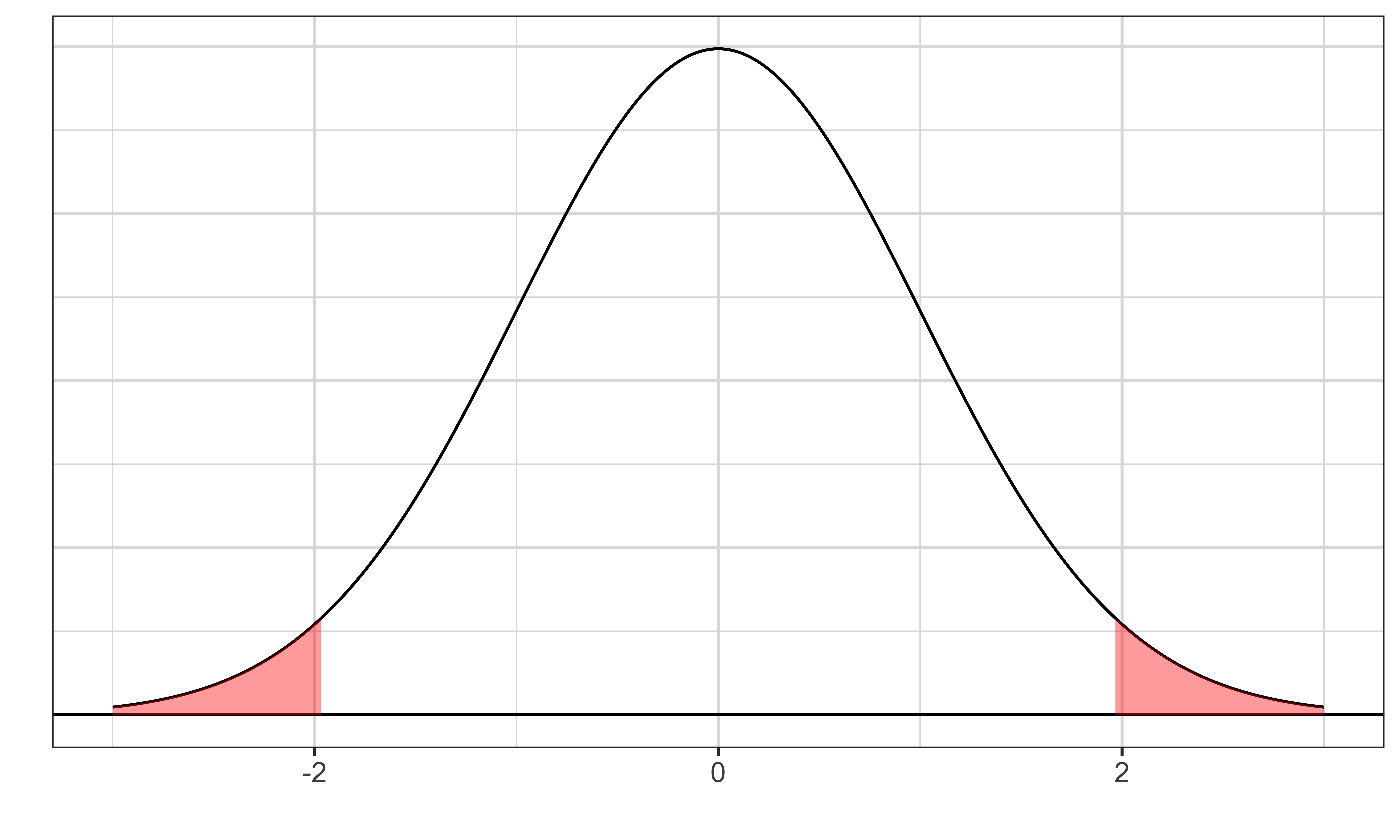
Now calculate the ninety-percent interval. Ninety percent in the center leaves ten percent outside, split evenly into five percent in each tail. We therefore need the five percent and ninety-five percent quantiles of a t distribution with five hundred and twenty-two degrees of freedom. The first interactive cell calls qt(0.05, df = 522) and qt(0.95, df = 522). The first argument is the cumulative probability and the named df argument selects the degrees of freedom. Running it returns symmetric values of about minus one point six four eight and positive one point six four eight.
The left column then states the central ninety-percent interval for the standardized statistic. Using the rounded values displayed in the fraction, the numerator is zero point five nine nine minus beta educ and the denominator is about zero point zero five one. That ratio lies between the two t quantiles in ninety percent of repeated samples under the model assumptions.
To translate back to beta educ, scale by the estimated standard error and shift by the estimate. The lower bound is zero point five nine nine plus zero point zero five one times minus one point six four eight. The upper bound is zero point five nine nine plus zero point zero five one times positive one point six four eight. Using the underlying unrounded values, the bounds are approximately zero point five one four and zero point six eight three. The negative lower quantile moves below the estimate; the positive upper quantile moves above it.
Look at the figure in the right column. Its horizontal axis is the t-statistic, its vertical height is the t density, and the red ribbons mark symmetric tail regions. The curve is symmetric and, with five hundred and twenty-two degrees of freedom, nearly indistinguishable from standard Normal. For the ninety-percent calculation on this tab, use the five and ninety-five percent quantiles printed by the interactive cell.
The final sentence hands you to the In practice tab. There, broom requests the same confidence level directly. Its conf.low and conf.high values should match the hand calculation.
Now, we need to find the 5% \big((100-90)/2\big) and 95% \big(100-(100-90)/2\big) quantiles of t_{522}.
So, \frac{0.599 - \beta_{educ}}{0.051} \sim t_{522} lies in [-1.648, 1.648] with probability 90% (before the sample is drawn)
By scaling and shifting, the lower and upper bounds of the 90% CI of \beta_{educ} are:
lower bound: 0.599 + 0.051 \times -1.648 = 0.514
upper bound: 0.599 + 0.051 \times 1.648 = 0.683
Confirm these against the In practice tab, which asks broom for the same interval.
The distribution of t_{522}:
Transcript
This is the practical way to obtain the interval from a fitted model. broom::tidy receives wage_reg as its first argument. Setting conf.int = TRUE asks broom to add confidence-interval endpoints to the usual coefficient table. Setting conf.level = 0.9 requests ninety-percent coverage rather than the common default of ninety-five percent. The decimal zero point nine is a proportion, not the number ninety.
The pipe sends the resulting tibble to dplyr::relocate(term, conf.low, conf.high). relocate does not change any calculations or rows. It simply moves the term name and the two interval columns to the front so they are easier to compare. The remaining columns, including estimate, standard error, statistic, and p-value, remain in the table after them.
Run the cell and find the educ row. conf.low is approximately zero point five one four and conf.high approximately zero point six eight three. These agree with the by-hand calculation on the previous tab, up to rounding.
You can just use broom::tidy() with conf.int = TRUE, conf.level = confidence level like below:
Multiple Linear Restrictions: F-test
Transcript
This baseball example introduces a joint hypothesis involving three restrictions. The dependent variable is log salary, where salary is measured in 1993. The model includes years in the league, average games played per year, career batting average, home runs per year, and runs batted in per year. Beta zero is the intercept and beta one through beta five multiply those regressors in the order shown.
The variable list supplies the substantive meanings. years measures career length, and gamesyr measures how regularly a player appears. We treat those as controls. The remaining variables measure performance: bavg is career batting average, hrunsyr is home runs per year, and rbisyr is runs batted in per year.
The question asks whether the three performance measures have any effect on salary collectively after holding years and games per year fixed. The word “collectively” is essential. H zero sets beta three, beta four, and beta five all equal to zero at the same time. Under that restriction, none of the three variables adds explanatory power conditional on the controls. There are q equals three restrictions.
H one says H zero is not true. That means at least one of those three coefficients is nonzero; it does not require all three to be nonzero, and it does not specify their signs. This is one joint hypothesis about a vector of parameters, not three independent yes-or-no questions. The next tab asks why we need a new testing device for this collective claim.
Model
log(salary) = \beta_0 + \beta_1 years + \beta_2 gamesyr + \beta_3 bavg + \beta_4 hrunsyr + \beta_5 rbisyr + u
- salary: salary in 1993
- years: years in the league
- gamesyr: average games played per year
- bavg: career batting average
- hrunsyr: home runs per year
- rbisyr: runs batted in per year
Hypothesis
Once years in the league and games per year have been controlled for, the statistics measuring performance ( bavg, hrunsyr, rbisyr) have no effect on salary collectively.
H_0: \beta_3=0, \beta_4=0, and \beta_5=0
H_1: H_0 is not true
Transcript
How should we test the joint null from the previous tab? The first bullet restates its logical structure: H zero holds only when beta three, beta four, and beta five are all zero. If even one is nonzero, the joint null is false. That makes it tempting to run an ordinary t-test for each coefficient and combine the three conclusions.
How do we test this?
- H_0 holds only if \beta_3, \beta_4, and \beta_5 are all zero.
- Conduct t-test for each coefficient individually?
Transcript
This cell loads the baseball data and fits the unrestricted model. data("mlb1", package = "wooldridge") loads mlb1 from the Wooldridge package. The model formula places log(salary) on the left and years, gamesyr, bavg, hrunsyr, and rbisyr on the right. The logarithm is applied within the formula. data = mlb1 supplies the observations, and the fitted fixest object is stored as mlb_reg.
The call to broom::tidy(mlb_reg) converts the coefficient results into a tibble and prints it. The cell has autorun: true, so the data and model objects are created for later tabs automatically. Ignore the comment’s spelling and focus on the model itself: this is the full, unrestricted specification because none of the three performance coefficients is forced to zero.
Read the output rows for bavg, hrunsyr, and rbisyr. Their estimates are approximately zero point zero zero zero nine eight, zero point zero one four four, and zero point zero one zero eight. Their estimated standard errors are roughly zero point zero zero one one zero, zero point zero one six one, and zero point zero zero seven one seven. Dividing each estimate by its standard error gives t-statistics of about zero point eight nine, zero point nine zero, and one point five zero.
The corresponding two-sided p-values are about zero point three seven six, zero point three six nine, and zero point one three four. These values concern each coefficient separately, conditional on all other regressors remaining in the model. Before moving on, ask whether those individual results logically establish that the three coefficients are jointly zero. The next Question and Answer tabs make the distinction explicit.
Transcript
The same tidy output appears again so you can inspect it without flipping back. Go row by row through bavg, hrunsyr, and rbisyr. For each one, compare its two-sided p-value with ten percent, zero point one zero. Batting average has a p-value around zero point three seven six, home runs per year around zero point three six nine, and runs batted in per year around zero point one three four.
None is below ten percent. Equivalently, none of the absolute t-statistics exceeds the two-sided ten-percent critical value. Thus every individual test fails to reject that coefficient equals zero while controlling for the other performance measures and the two career controls.
What do you find?
Transcript
The result is deliberately surprising: none of the coefficients on batting average, home runs per year, or runs batted in per year is individually statistically significant, even at the ten-percent level. “Individually” means each t-test asks whether one coefficient is zero while the other two performance variables remain in the regression. The data do not estimate any one variable’s unique partial effect precisely enough to reject zero at that threshold.
Do not convert those three decisions into the statement that performance collectively has no effect on salary. Failure to reject each coefficient separately is not evidence that all three population coefficients are exactly zero. The estimates may be correlated, and the group can carry substantial information even when the model cannot allocate that information precisely among its members.
The joint null is more demanding: beta bavg, beta hrunsyr, and beta rbisyr must all equal zero simultaneously. To evaluate it, compare the unrestricted model containing the three variables with a restricted model that imposes H zero by removing them. If the group contributes little, forcing the coefficients to zero should barely worsen the fit. If the group matters, the restricted model’s residuals should become substantially larger.
The slide points specifically to SSR, the sum of squared residuals, or equivalently a comparison based on R squared.
None of the coefficients on bavg, hrunsyr, and rbisyr is statistically significantly different from 0 even at the 10% level!!
So, does this mean that they collectively have no impact on the salary of MLB players?
If you were to conclude that they do not have statistically significant impact jointly, you would turn out to be wrong!!
SSR (or R^2) turns out to be useful for testing their impacts jointly.
In doing an F-test of the null hypothesis, we compare sum of squared residuals (SSR) of two models:
Unrestricted Model
log(salary) = \beta_0 + \beta_1 years + \beta_2 gamesyr + \beta_3 bavg + \beta_4 hrunsyr + \beta_5 rbisyr + u
Restricted Model
log(salary) = \beta_0 + \beta_1 years + \beta_2 gamesyr + u
The coefficients on bavg, hrunsyr, and rbisyr are restricted to be 0 following the null hypothesis.
Transcript
The slide above this tab defines the two models used by the F-test. The unrestricted model contains years, games per year, batting average, home runs per year, and runs batted in per year. The restricted model keeps only years and games per year. Dropping the three performance variables imposes the joint null that their coefficients are all zero.
The question asks which model should have the larger sum of squared residuals if we fit both to the same observations. Recall the OLS objective: choose coefficient values that minimize the sum of squared residuals. The unrestricted model may choose any values for all five slope coefficients. The restricted model is forced to choose beta three, beta four, and beta five equal to zero.
Think through the constrained-minimization logic, then open the Answer tab.
If the null hypothesis is indeed true, then what do you think is going to happen if you compare the SSR of the two models? Which one has a bigger SSR?
Transcript
The restricted model’s SSR must be at least as large as the unrestricted model’s SSR. The unrestricted OLS fit chooses coefficients from a larger set. It could reproduce the restricted fit exactly by setting the three performance coefficients to zero, so it can never do worse. It will do better whenever nonzero choices reduce the residual sum of squares.
The slide phrases this as the restricted model having smaller explanatory power, which is the intuition. More precisely, the restricted SSR is greater than or equal to the unrestricted SSR. Equality is possible if the restrictions do not change the sample fit. Therefore SSR sub r minus SSR sub u is always nonnegative for these nested models estimated on the same data with the same dependent variable.
SSR from the restricted model should be large because the restricted model has a smaller explanatory power than the unrestricted model.
SSR of the unrestricted model: SSR_u
SSR of the restricted model: SSR_r
Transcript
The code above this tab has fitted both nested models and printed their sums of squared residuals. The unrestricted fit includes all five regressors and stores its residuals in res_u. sum(res_u$residuals^2) squares every residual and adds the squares to obtain SSR sub u. The restricted fit includes only years and games per year, and the analogous expression obtains SSR sub r.
As predicted, the restricted number is larger. The question asks what the difference SSR sub r minus SSR sub u measures. Compare the formulas for the two regressions. They use the same dependent variable, same observations, same controls, and same OLS criterion. The only change is whether batting average, home runs per year, and runs batted in per year are allowed to enter.
What does SSR_r - SSR_u measure?
Transcript
SSR sub r minus SSR sub u is the reduction in residual sum of squares produced by adding the three excluded performance variables to the restricted model. In that sense, it measures their joint contribution to explaining log salary after years and games per year are already controlled for.
It is not the unique contribution of any single performance variable, and it is not generally the sum of three separate one-variable improvements. The regressors may overlap in the information they carry. The unrestricted model chooses all three coefficients together, so the SSR difference captures their combined ability to fit the dependent variable, including contributions that cannot be cleanly allocated when the variables are correlated.
The contribution from the three excluded variables in explaining the dependent variable.
Transcript
Now that we know what SSR sub r minus SSR sub u measures, ask whether the observed contribution is large enough to conclude that the excluded variables matter in the population.
Is the contribution large enough to say that the excluded variables are important?
Transcript
We cannot tell at this point because we do not know the null distribution of the raw difference SSR sub r minus SSR sub u. Computing a sample number completes only the calculation step. Without a reference distribution, words such as “large” or “unlikely” have no formal meaning.
This returns us to step two of the five-step recipe. We must ask what values an appropriately standardized improvement in fit would take if the three population coefficients were all zero. Under H zero, extra regressors can still reduce sample SSR by fitting random noise, so a positive improvement is expected. The question is whether the improvement is unusually large relative to that chance behavior.
Cannot tell at this point because we do not know the distribution of the difference!
Setup
Consider a following general model:
y = \beta_0 +\beta_1 x_1 + \dots+\beta_k x_k +u
Suppose we have q restrictions to test: that is, the null hypothesis states that q of the variables have zero coefficients.
H_0: \beta_{k-q+1} =0, \beta_{k-q+2} =0, \dots, \beta_k=0
When we impose the restrictions under H_0, the restricted model is the following:
y = \beta_0 +\beta_1 x_1 + \dots+\beta_{k-q} x_{k-q} + u
F-statistic
If the null hypothesis is true, then,
F = \frac{(SSR_r-SSR_u)/q}{SSR_u/(n-k-1)} \sim F_{q,n-k-1}
- q: the number of restrictions
- n-k-1: degrees of freedom of residuals
Transcript
Before using the general F formula above, check its sign. The statistic is open parenthesis SSR sub r minus SSR sub u close parenthesis divided by q, all divided by SSR sub u over n minus k minus one. Here q is the positive number of restrictions, and n minus k minus one is the positive residual degrees of freedom.
The denominator contains SSR sub u, a sum of squared residuals. Except for a perfect fit it is positive, and dividing by positive residual degrees of freedom preserves that sign. It estimates the error variance in the unrestricted model.
The numerator contains the difference between restricted and unrestricted SSR. For nested OLS models fitted on the same observations, the unrestricted model’s feasible coefficient choices include the restricted choices. Therefore the minimized unrestricted SSR cannot exceed the restricted SSR. The difference is nonnegative, and division by q leaves it nonnegative.
So what sign can F have? Recall that equality of the two SSR values is possible when the restrictions make no difference to the sample fit. Answer with that boundary case in mind, then open the Answer tab.
Is the above F-statistic always positive?
Transcript
The F-statistic is nonnegative. The restricted sum of squared residuals can never be below the unrestricted sum for nested OLS models estimated on the same sample, so SSR sub r minus SSR sub u is greater than or equal to zero. The remaining quantities in the ratio are positive under an ordinary nondegenerate regression.
If the restriction does not change the fitted values at all, the two SSR values are equal and F is exactly zero. Otherwise, the restricted fit is worse and F is positive. This is the constrained-minimum argument from the previous tabs, not an empirical pattern that happens only most of the time.
Yes, because SSR_r-SSR_u is always non-negative: the restricted model can never fit better than the unrestricted one.
Transcript
Read the F formula one more time to determine its direction. The numerator is the loss of fit from imposing q restrictions, averaged over those restrictions. The denominator is the unrestricted residual mean square, which measures the remaining noise per residual degree of freedom.
Choose between “greater” and “smaller” from the formula itself.
The greater the joint contribution of the q variables, the (greater or smaller) the F-statistic?
Transcript
Greater. When the q variables contribute more jointly, removing them increases the restricted model’s residual sum of squares by more. The gap SSR sub r minus SSR sub u becomes larger. After dividing by q and by the unrestricted residual mean square, that larger standardized loss produces a larger F-statistic.
A small F has the opposite interpretation. It says the restricted and unrestricted models fit similarly after accounting for the number of restrictions and noise. Dropping the variables cost little, so the data are compatible with their coefficients being jointly zero. We then fail to reject H zero.
Greater.
Transcript
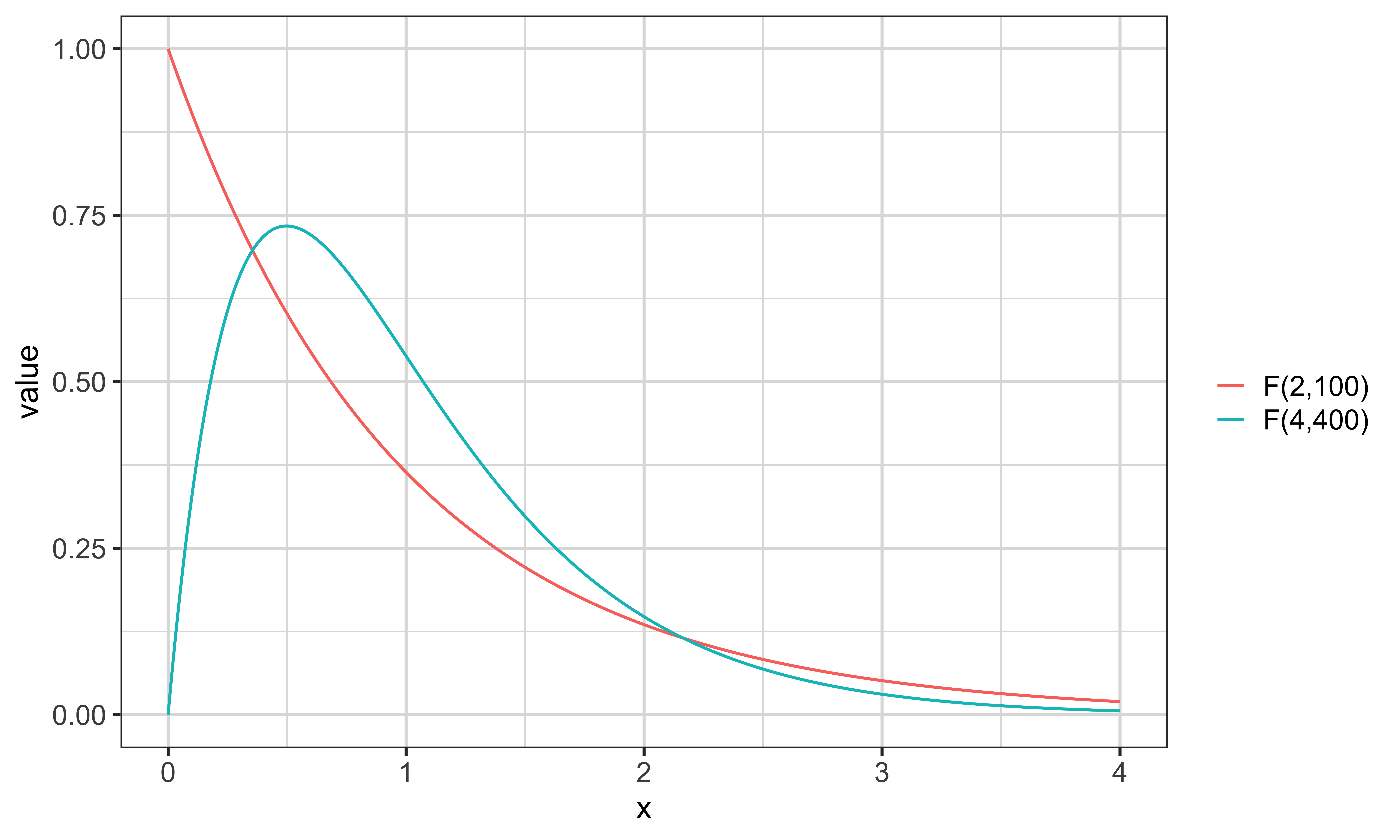
This slide puts the F reference distribution beside the testing recipe. Start with the figure on the left. The horizontal axis shows nonnegative F values and the vertical axis shows probability density. The two curves are different F distributions: F with two numerator and one hundred denominator degrees of freedom, and F with four numerator and four hundred denominator degrees of freedom. Both are right-skewed and live only on zero and positive values, consistent with the SSR-ratio construction. Their shapes differ because an F distribution requires two degrees-of-freedom parameters, so there is no single universal F curve.
Now read the five steps on the right. First define H zero precisely, including every restriction. Second estimate the unrestricted model and the restricted model on the same observations, then obtain SSR sub u and SSR sub r. The unrestricted model contains all coefficients; the restricted model imposes H zero. Third calculate F as the average SSR increase per restriction divided by the unrestricted residual mean square.
Fourth choose a significance level and find the matching upper-tail critical value from F with q numerator degrees of freedom and n minus k minus one denominator degrees of freedom. Here q is the number of restrictions and k counts regressors in the unrestricted model excluding its intercept.
Fifth compare the observed statistic with the critical value. Reject H zero if F is greater, because only a large standardized loss of fit is evidence that the restrictions are false. Otherwise fail to reject. This is the same general five-step logic from the first slide, specialized to a statistic that tests several linear restrictions at once. The next tabs implement each calculation for the baseball model.
F-distribution
F-test steps
- Define the null hypothesis
- Estimate the unrestricted and restricted models to obtains their SSR
- Calculate F-statistic
- Define the significance level and corresponding critical value according to the F distribution with appropriate degrees of freedoms
- Reject if your F-statistic is greater than the critical value, otherwise do not reject
Transcript
Step one fits the two nested models and obtains their sums of squared residuals. In the unrestricted call, feols regresses log salary on years, games per year, batting average, home runs per year, and runs batted in per year, using mlb1. The line break after gamesyr + is only formatting; the plus sign continues the formula. The fitted object is stored as reg_u.
reg_u$residuals extracts the vector of unrestricted residuals. Raising it to the second power squares each element, and sum adds those squares. The result is stored as SSR_u. This is the minimized residual sum of squares when all five slope coefficients are free.
The restricted call regresses the same log salary outcome on only years and games per year. It uses the same dataset and estimator but omits bavg, hrunsyr, and rbisyr, thereby imposing the three zero restrictions in H zero. The fitted object is reg_r, and squaring and summing reg_r$residuals gives SSR_r.
Compare the formulas carefully. The dependent variable, observations, controls, intercept treatment, and OLS method are identical. Only the three jointly tested variables differ. That nested structure is required for interpreting SSR sub r minus SSR sub u as the fit lost by imposing the null. Both model cells use earlier-loaded data, and autorun: true ensures the objects exist for Step 2, where the raw gap is converted into an F-statistic.
Estimate the unrestricted and restricted models
Transcript
Step two assembles the F-statistic from the objects created in Step 1. df_q <- 3 records q, the number of restrictions: one each for batting average, home runs per year, and runs batted in per year. It is not a residual degree of freedom; it will be the numerator degrees of freedom of the F distribution.
degrees_freedom(reg_u, "resid") asks the unrestricted model for its residual degrees of freedom and stores the answer as df_ur. The unrestricted model is the relevant one because its SSR estimates the remaining error variance after all coefficients are freely estimated. With the available baseball observations and five regressors plus an intercept, this value is n minus five minus one.
F_stat_num <- (SSR_r - SSR_u) / df_q calculates the numerator mean square. Subtracting measures the fit lost under the restrictions, and dividing by three expresses the average loss per restriction. F_stat_denom <- SSR_u / df_ur calculates the unrestricted residual mean square. Under homoskedastic classical assumptions, this is sigma hat squared, the estimator of the error variance.
Finally, F_sta <- F_stat_num / F_stat_denom divides the restriction mean square by the residual mean square, and the last line prints F_sta. The ratio is unit-free because both pieces are measured in squared dependent-variable units. A value near the ordinary null range means the fit loss is modest relative to noise; a large value means the restrictions caused an unusually costly loss. Step 3 will use qf to decide how large is large at the chosen significance level.
Calculate F-stat
Transcript
Steps three and four choose the threshold and make the decision. alpha <- 0.05 sets the significance level to five percent. In this upper-tail test, the rejection region occupies the largest five percent of F values, so the critical value has ninety-five percent of the null distribution to its left.
qf(1 - alpha, df1 = df_q, df2 = df_ur) computes that boundary. qf is the F quantile function. Its first argument is zero point nine five. df1 receives the three numerator degrees of freedom, one per restriction, and df2 receives the unrestricted residual degrees of freedom. The result is assigned to c_value and printed. Do not divide alpha by two, because F is nonnegative and only the upper tail is a rejection region.
The second cell evaluates F_sta > c_value. This logical comparison returns TRUE for the baseball data, meaning the observed F-statistic lies beyond the five-percent critical value. Equivalently, its upper-tail p-value is below zero point zero five. We reject the joint null that all three performance coefficients are zero.
Read the Observation callout carefully. The variables have statistically significant impacts jointly, even though none of their individual two-sided t-tests rejected at ten percent. That is not a logical contradiction.
Find the critical value
Is F-stat > critical value?
Transcript
This is the practical interface for joint tests. marginaleffects::hypotheses receives the fitted unrestricted regression and the names of the coefficients that are all zero under H zero, then computes the joint F statistic from the model’s coefficient estimates and variance-covariance matrix. For a classical OLS model and restrictions that set a group of coefficients to zero, this is the same F statistic as the restricted-versus-unrestricted comparison we developed by hand. You do not have to estimate the restricted model yourself.
The syntax block has three arguments. regression is the fitted model object containing the unrestricted specification. joint is a character vector of coefficient names, written exactly as they appear in the regression output. Every coefficient listed there is set to zero under H zero, so the number of names is q, the number of restrictions. joint_test = "f" asks for the F-test; without it, the function reports a chi-squared version of the test instead. Because the code chunk has eval = F, it only illustrates syntax and does not try to execute placeholder names.
In the example, c("x1", "x2") uses c to create a character vector with two names, so it tests H zero: the coefficients on x1 and x2 are both zero, with q equal to two. Quotation marks matter because these are names the function looks up in the model, not R objects. Flip to the Demonstration tab to apply the function to the three baseball restrictions.
You can use the hypotheses() function from the marginaleffects package.
Syntax
regression: the name of the regression results of the unrestricted modeljoint: names of the coefficients that are all 0 under H_0. For example,c("x1", "x2")means H_0: \beta_{x1} = 0 and \beta_{x2} = 0joint_test = "f": report the F-test (the default is a \chi^2 test)
Transcript
This code applies the convenience function to the baseball regression. mlb_reg is the unrestricted model containing years, games per year, batting average, home runs per year, and runs batted in per year. The joint argument is a character vector made with c, containing "bavg", "hrunsyr", and "rbisyr". Setting those three coefficients to zero is exactly the null stated at the start of the section, so q equals three. joint_test = "f" asks for the F-test.
hypotheses reads the coefficient names from the model, and its output first lists the three restrictions it tested, bavg equals zero, hrunsyr equals zero, and rbisyr equals zero, so you can confirm it tested what you intended. Below that it reports the F statistic, about nine point five five, its p-value, printed as less than zero point zero zero one, and the two degrees of freedom: three, the number of restrictions q, and three hundred forty-seven, which is n minus k minus one for this model.
Compare this with the by-hand F calculation. The F statistic is the same, nine point five five, and so are the degrees of freedom, because under the classical assumptions this is the same test. The p-value is far below five percent, so the joint null is rejected: the performance variables matter collectively, even though none of them was individually significant.
The following code tests if \beta_{bavg} = 0, \beta_{hrunsyr} = 0, and \beta_{rbisyr} = 0.