01-1: Univariate Regression: Introduction

Univariate Regression: Introduction


Population, Sample, and Econometrics

Transcript

Everything in econometrics starts with a question about a population, so let’s be precise about that word. A population is the complete set of people, farms, firms, objects, or outcomes you want your conclusion to describe. The red word “ALL” in the definition is doing real work. The population is not just the cases you happened to observe, and it is not automatically everyone who exists.

Look at the first example. If your question is the effect of education on income across the United States, the population is all individuals in the United States who fall within the scope of that question. In the second example, the units are farmers rather than individuals, the outcome is irrigation water demand, and the geographic scope is Nebraska. That makes all Nebraska farmers the population of interest.

Now read the Important block. The population is determined by the question you ask. If the question concerns COVID-19 and children’s educational achievement globally, every child in the world is in scope. If you narrow the question to the United States, children outside the United States leave the target population. That distinction matters because an estimate can only be interpreted relative to a stated population. Later, when we discuss sampling and external validity, you will ask whether the observed sample supports a conclusion about that full target group. Before doing any regression, you should therefore be able to finish this sentence clearly: “I want to learn about all of these units.” Flip to the Sample tab to see the much smaller set we actually observe.

Definition

A set of ALL individuals, items, or phenomena that you are interested in learning about


Example

  • Suppose you are interested in the impact of education on income across the U.S. Then, the population is all the individuals in U.S.
  • Suppose you are interested in the impact of water pricing on irrigation water demand for farmers in NE. Then, your population is all the farmers in NE.

Important

Population differs depending on the scope of your interest

  • If you are interested in understanding the impact of COVID-19 on child education achievement at the global scale, then your population is every single kid in the world

  • If you are interested in understanding the impact of COVID-19 on child education achievement in U.S., then your population is every single kid in U.S.

Definition

Sample is a subset of population that you observe

Transcript

A sample is the subset of the population that you actually observe. Here the population question concerns the effect of education on wages, while the sample contains education, income, and other characteristics for three hundred people from each state. Those observed people are the units that will enter your calculations. Everyone else in the population remains unobserved.

The note asks whether this sample is representative of the population. “Representative” means that the sample supports the population-level comparison you want to make, not merely that it contains many observations or includes every state. This particular design gives each state exactly three hundred observations. That may be useful if you want reliable state-by-state comparisons, but it does not mirror the national population. A person from a small state has a much larger chance of appearing than a person from a large state, so an unweighted national average would give small and large states equal sample influence even though their populations differ greatly. Appropriate sampling weights might repair that mismatch for some national summaries, but only if the sampling design and response process are understood.

Also ask who within each state was selected and who responded. A random sample from a complete list has a different interpretation from a convenience survey of volunteers. The software can compute a regression either way, but it cannot decide whether the observed people stand in for the population you named. That is a research-design judgment. Case 2 makes the same issue even more visible by narrowing the observed geography.

  • Population: you are interested in the impact of education on wage
  • Sample (example): data on education, income, and many other things for 300 individuals from each State

Question

Is the sample representative of the population?

Transcript

Now the second case, where the mismatch between population and sample is geographic. The population named in the first bullet is all farmers in Nebraska because the research question asks how Nebraska farmers’ irrigation responds to water prices. The sample in the second bullet is only five hundred farmers in the Upper Republican Basin, in the southwest corner of the state. For those farms you observe water price, irrigation water use, and other characteristics.

The question in the note is again whether the sample is representative of the stated population. Farmers in one basin may share climate, soils, groundwater conditions, crop choices, irrigation technologies, and water regulations that differ from conditions in central or eastern Nebraska. Any of those differences can change water demand or change how farmers react to a price. A careful estimate may describe the sampled basin very well and still fail to describe the entire state. A large sample does not solve that problem, because five hundred observations drawn from the wrong slice of the target population can give a very precise answer to a narrower question.

This is not a reason to discard the data. You could redefine the target population as farmers in the Upper Republican Basin, or you could make and defend an argument that the response found there transports to other Nebraska farmers. What you may not do is silently move from the observed basin to the whole state. The population determines whom the conclusion is about; the sample determines the evidence you actually have. Keep that distinction in mind as we move from data collection to the population regression model we want the sample to reveal.

  • Population: you are interested in the impact of water price on irrigation by farmers in Nebraska
  • Sample (example): data on water price, irrigation water use, and many other things for 500 farmers who farm in the Upper Republican Basin (southwest corner of NE)

Question

Is the sample representative of the population?

Simple univariate model

Transcript

Here is the object the rest of this course is built on. Read the equation aloud as “y equals beta zero, plus beta one times x, plus u.” It is a model of a phenomenon in the population, not yet an estimated line from a sample. The slide asks us to suppose that this model correctly represents the population relationship we want to learn about.

Work through the four bullets. The dependent variable, y, is the outcome to be explained. It might be income, corn yield, or irrigation water use. The variable x is used to explain y. You will hear x called the independent variable, covariate, or explanatory variable; on this slide those names refer to the same role. The error term, u, contains every part of y that x does not explain. That includes omitted influences, individual circumstances, and unpredictable shocks. Calling it an error does not mean somebody made a data-entry mistake.

Beta zero and beta one are population parameters, fixed real numbers that give the model quantitative meaning. Beta zero locates the line, and beta one determines how y changes with x. They are not random across observations in this model. By contrast, x and u vary from one unit to another, which makes y vary as well.

The blue phrase and the final callout identify the econometric problem. This true population model is the object you want to know, but you do not observe the population equation or its true parameter values. You observe a sample of x and y values and use statistics to estimate the betas. The next two tabs explain exactly what each parameter means before we try to estimate either one.

Consider a phenomenon in the population that is correctly represented by the following model ( This is the model you want to learn about using sample ):

\begin{equation*} y=\beta_0+\beta_1 x + u \end{equation*}
  • y: to be explained by x ( dependent variable)
  • x: explain y ( independent variable , covariate , explanatory variable )
  • u: parts of y that cannot be explained by x ( error term )
  • \beta_0 and \beta_1: real numbers that gives the model a quantitative meaning ( parameters )

Important

You will never know the true model. You can try estimating it using sample! That is what statistics is about.

Transcript

Beta one is the slope, but the equations show exactly what that means. Start with the first line, “y equals beta zero, plus beta one times x, plus u.” Now imagine changing x by one unit while holding u constant. The before outcome is beta zero, plus beta one times x, plus u. The after outcome replaces x with x plus one, while beta zero and the same u remain unchanged.

To see the last displayed line, subtract y before from y after. Expanding beta one times x plus one gives beta one times x, plus beta one. The beta-zero terms cancel, the beta-one-times-x terms cancel, and the identical u terms cancel. The only term left is beta one. Therefore delta y, meaning y after minus y before, equals beta one.

Pay attention to units. If x is kilograms of fertilizer per hectare and y is bushels per acre, beta one is the change in bushels per acre associated with one additional kilogram of fertilizer per hectare. If x rises by two units in this linear model, y changes by two times beta one. A positive beta one means y rises; a negative beta one means y falls; zero means no change in the modeled outcome.

The phrase in blue, ceteris paribus, means “with everything else fixed.” Holding u fixed prevents rainfall, ability, soil quality, or any other omitted influence from changing at the same time as x. Without that comparison, a difference in y could combine the effect of x with changes in those other factors. The callout therefore describes beta one as the ceteris paribus causal impact. Learning that causal quantity from observational data requires conditions that make comparisons across x behave like this imagined one-factor change. That difficulty motivates the college example after the visual interpretation.

\begin{align*} y=\beta_0+\beta_1 x + u \end{align*}

If you change x by 1 unit while holding u (everything else) constant,

\begin{align*} y_{before} & = \beta_0+\beta_1 x + u \\ y_{after} & = \beta_0+\beta_1 (x + 1) + u \end{align*}

The difference in y_{before} and y_{after},

\begin{align*} \Delta y = \beta_1 \end{align*}

That is, y changes by \beta_1.

So,

  • \beta_1 is the change in y when x increases by 1
  • We call \beta_1 the ceteris paribus (with everything else fixed) causal impact of x on y.
Transcript

Beta zero is the intercept. Algebraically, look at the first equation and set x equal to zero. The beta-one-times-x term then vanishes, leaving y equal to beta zero plus u. If we also set u equal to zero, as the next line does, y equals beta zero. Geometrically, beta zero is therefore the height of the population line when x is zero.

The following sentence gives a related average interpretation, but it depends on a condition. Take the conditional expectation of the model at x equal to zero. The result is expected y given x equals zero, equals beta zero plus expected u given x equals zero. Under the zero conditional mean condition, expected u given x is zero for every x, including zero. Only then does beta zero equal the average value of y among population units with x equal to zero. We will define and examine that condition in the Crucial condition tab.

Now read the note, because an intercept can be mathematically necessary without having an interesting substantive story. Suppose x is years of education in a sample containing only people with ten to twenty years of education. Beta zero predicts income at zero years, far outside the observed range. That is extrapolation, so the number may be unrealistic and is not supported directly by the data. If x is a treatment indicator that equals zero for a real control group, however, the intercept can be meaningful as that group’s expected outcome under zero conditional mean.

We normally keep the intercept even when zero is not substantively useful. Omitting it forces the fitted relationship through the origin, asserting that y must be zero whenever x is zero. That is a strong restriction and can distort the slope. So interpret beta zero when zero is meaningful, but do not remove it merely because its story is uninteresting.

\begin{align*} y=\beta_0+\beta_1 x + u \end{align*}

When x = 0 and u=0,

\begin{align*} y=\beta_0 \end{align*}

So, \beta_0 represents the intercept.

Under the zero conditional mean condition E[u|x]=0 (see the Crucial condition tab in the next section), \beta_0 = E[y|x=0]: the average value of y among those with x=0.

Note

\beta_0 is most useful when x=0 is substantively meaningful and within the observed range. Otherwise it is an extrapolation. The intercept should normally remain in the model so the regression is not forced through the origin, but it may not deserve a substantive story.

Transcript

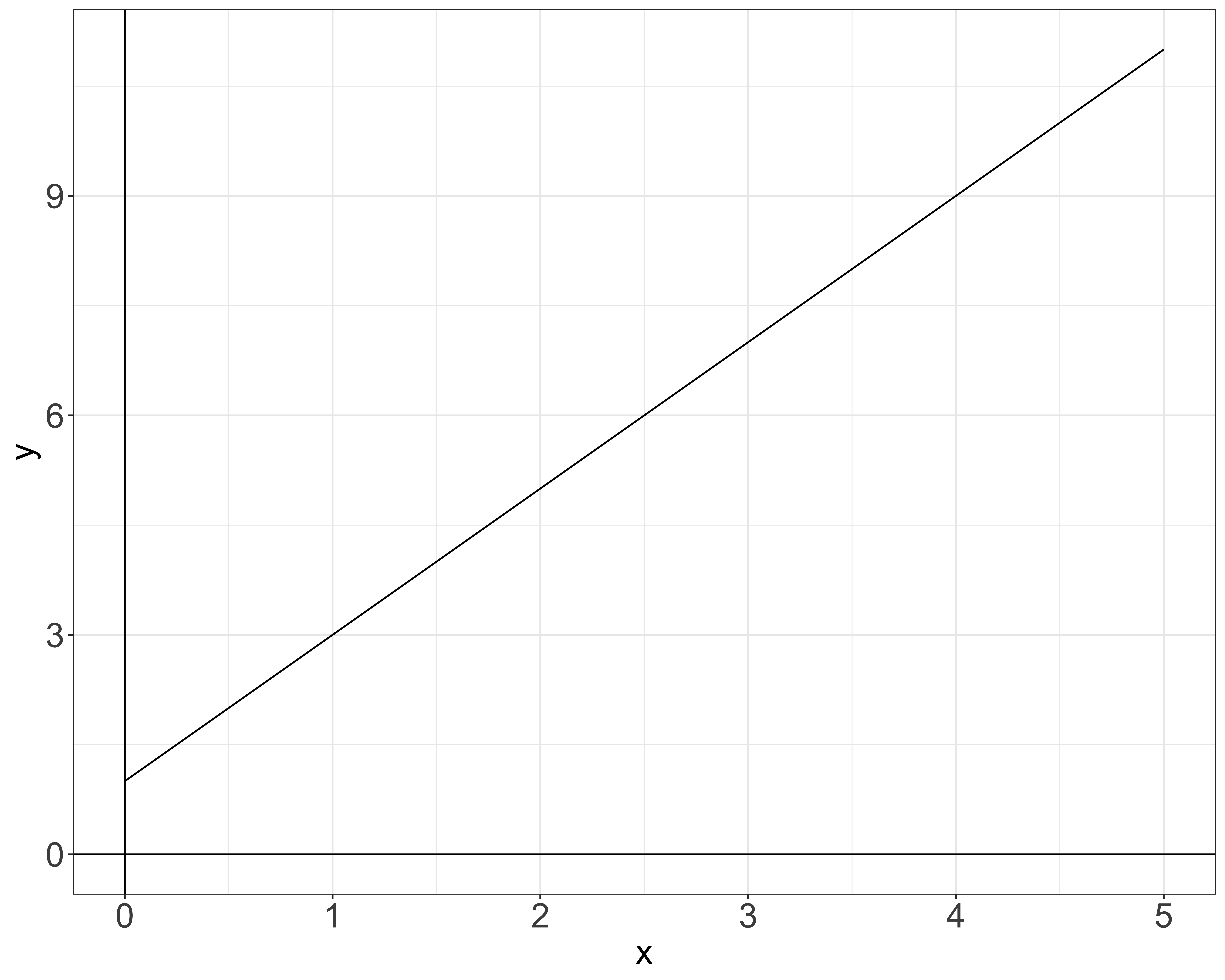
Now connect the two parameters to the picture. The horizontal axis is x, running from zero to five, and the vertical axis is y. The plotted line follows y equals one plus two times x, so this illustration has beta zero equal to one and beta one equal to two. There are no scattered observations or error terms in this figure; it is showing the systematic line itself.

Start at x equal to zero. The blue point marks where the line crosses the vertical axis, at y equal to one. That is beta zero, the intercept. You can verify other points from the equation: when x is two, y is one plus two times two, which is five. When x is three, y is seven.

The red right-angle step visualizes beta one. Its horizontal segment moves from x equal to two to x equal to three, a one-unit increase in x, while beginning at y equal to five. Its vertical segment then rises from y equal to five to y equal to seven, a two-unit increase in y. Rise divided by run is two divided by one, so the slope is two. Because the model is linear, the same one-unit move produces the same two-unit rise anywhere along the line.

The left column calls beta one the coefficient or slope and beta zero the intercept. Keep both the algebra and this geometry together: beta zero sets the starting height, while beta one sets the direction and steepness. In the next lecture, the points will be scattered because u varies across observations. Estimation will then ask which intercept and slope place a line through those observed data in a principled way.


  • \beta_0: intercept
  • \beta_1: coefficient (slope)

Why do we want ceteris paribus causal impact?

Transcript

Let’s make ceteris paribus concrete with a decision you might actually face. The first three bullets set it up. You have been admitted to University A, described here as better and more expensive, and University B, described as worse and less expensive. You need to choose one, and the relevant benefit is the boost each school would give your future income. This is an individual causal question: how would your income differ if you attended A rather than B?

The table is observational evidence you found about former students. Each row is a university. “Average income” is the sample mean of graduates’ annual incomes, and “sample size” is the number of observed graduates. The displayed data contain five hundred graduates from each school. With the fixed simulation used for this slide, A’s mean income is 131.26 and B’s is 90.31, so the observed difference, A minus B, is 40.94 in the income units used here.

The question at the bottom asks whether you should treat that 40.94 as the expected boost that you personally would receive by attending A instead of B. Be careful about the comparison. The table compares two groups of different people who made different choices and passed different admissions processes. It does not observe the same person attending both schools. Your causal question instead compares two potential outcomes for you, one under A and one under B, with your own characteristics held fixed.

The raw difference could reflect what A does, but it could also reflect who attends A. A more selective university may enroll students who would have earned more regardless of where they studied. The table alone cannot separate those explanations. Keep 40.94 in mind, then flip to the next tab, where we state the comparison you actually want.

Quality of College

You

  • have been admitted to University A (better, more expensive) and B (worse, less expensive)
  • are trying to decide which school to attend
  • are interested in knowing a boost in your future income to make a decision

You have found the following data

University

average income

sample size

A

131.26

500

B

90.31

500

Question

Should you assume that the observed difference of 40.94 is the expected boost you would get if you are to attend University A instead of B?

Transcript

Here are two quantities, and the distinction between them is the heart of the lecture. Suppose your ability score is six out of ten. The first expression is expected income conditional on attending A, minus expected income conditional on attending B. Read expected income given A as the average income among people who attend A, and similarly for B. This is the raw group difference from the table, about 40.94.

The second expression adds ability equal to six to both conditioning sets. It compares expected income at A for people with ability six with expected income at B for people with ability six. School changes, but ability is deliberately held fixed at your level. That is the quantity relevant to your decision because you do not become a different person when we imagine sending you to the other school.

The first callout bullet explains why this restriction matters. Innate ability does not miraculously increase simply because you enroll at A. If A’s students tend to have greater ability before college, then the first expression changes school and ability together. The second callout bullet names the problem: the school effect is confounded with something else. A confounder affects income and is systematically related to school attendance, so its contribution becomes mixed into the raw school comparison.

The note at the bottom defines the notation. Expected Y given X means the average value of Y for units with a specified value of X. Conditioning on more variables creates a more like-for-like comparison. Here we condition on both school and ability so that we compare students of equal ability across schools. Of the two displayed quantities, you want number two, the ceteris paribus difference. The next tab shows why the two quantities differ in the observed data.

Let’s say your ability score is 6 out of 10 (the higher, the better),

\text{(1)}\;\; E[inc|A] -E[inc|B] \;\;\; \text{(the raw difference in the table)} \text{(2)}\;\; E[inc|A,ability=6] -E[inc|B,ability=6]

Which one would you like to know?

Important

  • You want ability (an unobservable) to stay fixed when you change the quality of school because your innate ability is not going to miraculously increase by simply attending school A

  • You do not want the impact of school quality to be confounded with something else

Aside: Conditional Expectation

E[Y|X] represents expected value of Y conditional on X (For a given value of X, the expected value of Y).

Transcript

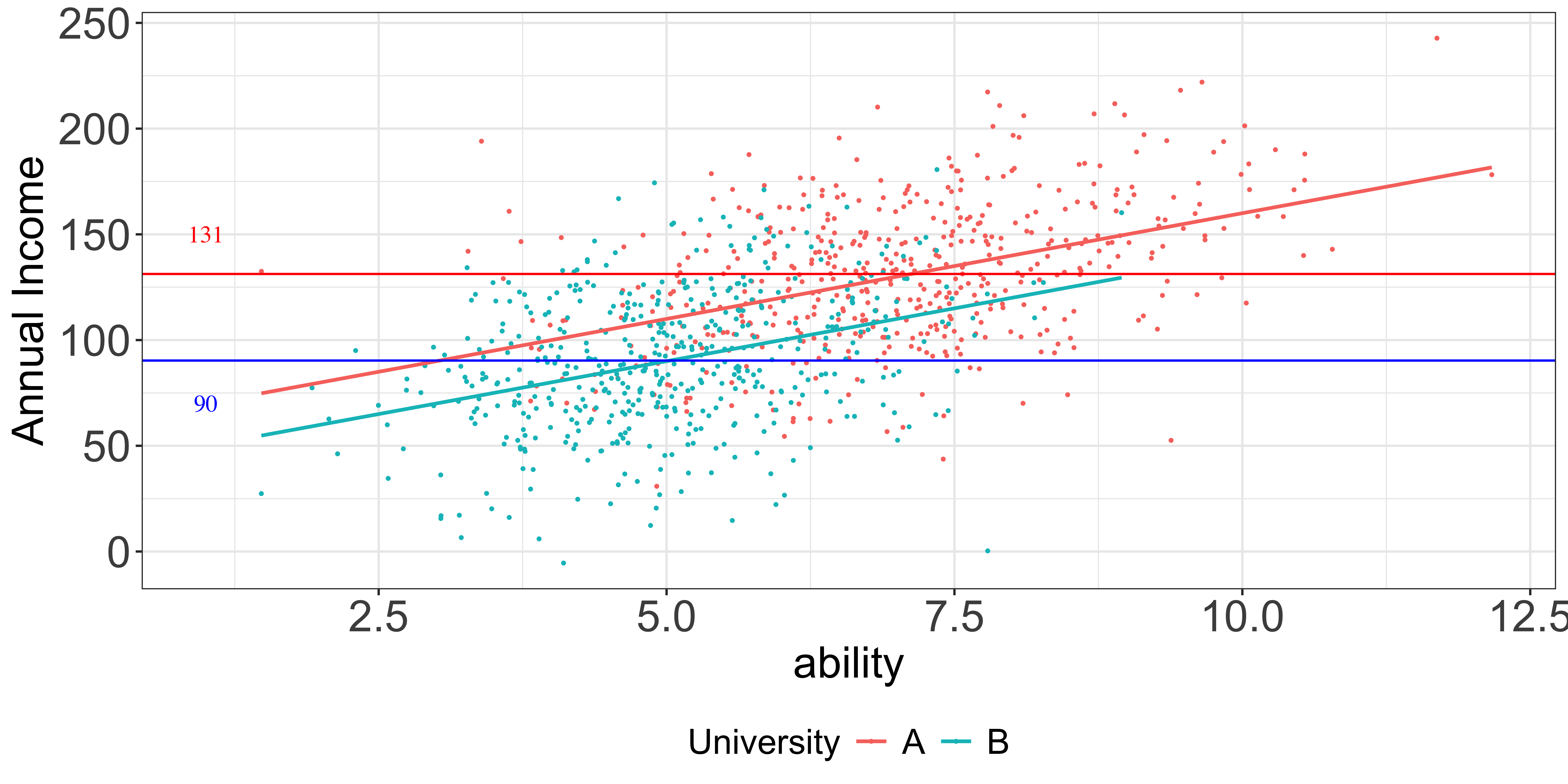
Now look at what is actually in the data. Each dot represents one graduate. The horizontal axis is ability, with higher values farther to the right, and the vertical axis is annual income. Color identifies the university. The red cloud and red lines correspond to University A; the blue cloud and blue lines correspond to University B.

The sloped lines show expected income conditional on both university and ability, exactly as the note says. At any fixed ability, draw an imaginary vertical line upward. The red University A line is twenty income units above the blue University B line. Because the lines are parallel, that conditional gap is twenty at every displayed ability value. This is the ceteris paribus school effect built into the example.

The horizontal lines show something different: each university’s overall sample mean income, ignoring ability. The red horizontal line is around 131 and the blue horizontal line is around 90, so their separation is about 41. Those are the numbers from the previous table. Their gap is much larger than the vertical distance between the sloped lines.

The distribution of dots explains why. University A’s red observations are concentrated farther to the right, around ability seven, while University B’s blue observations are concentrated farther left, around ability five. Ability raises income within either school, as shown by the positive slope of both conditional lines. Consequently, A’s overall average income is high for two reasons: A has a positive school effect, and A enrolls students with higher average ability. The horizontal-line comparison mixes those reasons. The sloped-line comparison holds ability fixed and isolates the school effect. Flip to the next tab to put exact numbers on those two components.
Note

  • red line: E[income|A, ability]
  • blue line: E[income|B, ability]

Transcript

Let’s put numbers on the picture, because the size of the mistake matters. University A’s students have an average ability of about 7.0, and University B’s have an average of about 5.0. Within either school, each one-point increase in ability raises expected income by ten. A two-point average ability difference therefore contributes roughly twenty income units to the raw difference between the groups.

At any fixed ability, compare the formulas behind the sloped lines. For A, expected income is sixty plus ten times ability. For B, it is forty plus ten times ability. Subtract B from A while holding ability constant. The ten-times-ability terms cancel, leaving sixty minus forty, which is twenty. That is the ceteris paribus effect of attending A in this example.

Now read the three bullets. Number one is the gap between the horizontal group-mean lines, about 40.9 in this realized sample. That is what you see when you compare graduates without controlling for ability. Number two is the twenty-unit gap between the sloped conditional-mean lines. That is what attending A does for a student of any given ability. The remaining 20.9 is the raw gap minus twenty. It reflects the groups’ different ability composition plus sampling noise, not the effect of the school itself.

The exact decomposition is especially clear at the population means: roughly twenty comes from A’s school premium and roughly twenty comes from its two-point ability advantage. The random noise in observed incomes makes the sample values differ slightly from those round numbers. The fragment gives the practical consequence. If you credit A with the entire raw difference, you value it at about twice its true twenty-unit effect. The rest of the course develops research designs and estimators that try to recover the conditional, like-for-like comparison from data that initially offer only raw differences.

A’s students average an ability of 7, B’s average 5, and each point of ability is worth 10 of income. At the same ability, A pays 60 and B pays 40.

  • (1) the gap between the two horizontal lines is 40.9   ← what you see
  • (2) the gap between the two sloped lines is 20   ← what attending A does for you
  • the remaining 20.9 is ability, not school

Important

Take (1) at face value and you credit University A with roughly twice what it is worth. The whole of this course is machinery for getting from (1) to (2).

Example: corn yield and fertilizer

Transcript

Let’s switch to an agricultural example and practice identifying the error term in a real setting. Read the equation as “yield equals beta zero, plus beta one times fertilizer, plus u.” Yield is the dependent variable, measured for a field or farm. Fertilizer is the explanatory variable, ideally with a clearly stated unit such as kilograms of nitrogen per hectare. Beta zero is the modeled yield when fertilizer and the error are zero, and beta one is the change in yield associated with one additional unit of fertilizer while everything in u is held fixed.

The question asks what belongs in u. By definition, u contains every determinant of yield that is not represented by the fertilizer term. Plausible examples include rainfall, temperature, soil organic matter, soil texture, drainage, pest and disease pressure, seed variety, planting date, irrigation, machinery, farmer skill, and unexpected weather shocks. Measurement error in yield or fertilizer may also affect the disturbance represented by the error term, although its consequences require more careful treatment later.

Do not put an arbitrary characteristic into u merely because it was not recorded. A farmer’s favorite color belongs there only if it actually affects yield or is connected to an omitted yield determinant in the way the model represents. Conversely, an important factor remains part of u even if the researcher wishes it were irrelevant. The error term is defined by the gap between the outcome and the systematic part of the model, not by the contents of the dataset.

This list is usually long, and many entries are difficult or expensive to measure. That is normal. Econometrics does not require us to observe every determinant of yield, but it does require us to understand how those unobservables relate to fertilizer. The next tab states the estimation problem created by that relationship.

Corn yield and fertilizer

\begin{align*} yield=\beta_0+\beta_1 fertilizer+u \end{align*}

Question

What is in the error term?

Transcript

Here is the position you are in as an empirical researcher. The population model at the top still says yield equals beta zero, plus beta one times fertilizer, plus u. Beta zero and beta one belong to that population model, so you do not know their true values. Your task is to use sample evidence to estimate them.

The second bullet describes that evidence. For each observational unit i, running from one through n, you observe a pair: yield sub i and fertilizer sub i. The subscript identifies the field or farmer. Together, the n pairs tell you how yield and fertilizer co-vary in the sample. They do not directly reveal u sub i, because u contains the other yield determinants that were not observed or included.

The third bullet states the target. You want beta one to measure the ceteris paribus impact of fertilizer on yield, meaning the change caused by one more unit of fertilizer with rainfall, soil, management, pests, and all other factors held fixed. Simply drawing a line through observed yield and fertilizer pairs is not automatically enough. If high-fertilizer fields also have better soil or more skilled managers, the observed slope can credit fertilizer for their effects. If farmers apply more fertilizer to poor fields, the same raw slope can conceal part of fertilizer’s benefit. The direction depends on how fertilizer is related to the omitted factors.

That makes the question at the bottom sound impossible: how can we hold constant variables we do not observe? The key is that causal estimation does not always require every omitted influence to be measured individually. It requires a condition on how their average behaves across fertilizer levels. The next tab states that condition formally.

\begin{align*} yield=\beta_0+\beta_1 fertilizer+u \end{align*}
  • you do not know \beta_0 and \beta_1, and would like to estimate them
  • you observe a series of \{yield_i,fertilizer_i\} combinations (i=1,\dots,n)
  • you would like to estimate \beta_1, the impact of fertilizer on yield, ceteris paribus (with everything else fixed)

Question

How could we possibly find the ceteris paribus impact of fertilizer on yield when we do not observe whole bunch of other factors (error term)?

Transcript

The crucial condition is the line in the first callout: expected u given x equals zero. This is called zero conditional mean. The vertical bar means “given,” so for every value of x, the average error among population units with that x value must be zero. It does not require every individual error to be zero. Some high-fertilizer fields can have positive unobserved advantages and others negative disadvantages, as long as those omitted influences average to zero at that fertilizer level.

Here is why the condition identifies the regression function. Start from y equals beta zero, plus beta one times x, plus u, and take the expected value conditional on x. Beta zero is fixed. Once x is given, beta one times x is also fixed. Therefore expected y given x equals beta zero, plus beta one times x, plus expected u given x. Under the condition in the callout, the last term is zero. What remains is expected y given x equals beta zero plus beta one times x. Changes in the conditional mean of y across x then reveal beta one rather than a mixture of beta one and changing average unobservables.

In the fertilizer example, the condition says that fields receiving any particular fertilizer rate have, on average, no positive or negative bundle of omitted yield determinants. Equivalently, the average content of the error term cannot systematically move with fertilizer. That is the formal version of holding the rest of the world fixed in expectation.

The next paragraph states a sufficient formulation: if expected u given x always equals the unconditional expected u, then u is mean independent of x. With an intercept, we can normalize that common unconditional mean to zero, producing zero conditional mean. The final callout guards against two common mistakes. Zero conditional mean implies zero covariance between u and x, but zero covariance alone permits nonlinear dependence and is weaker. Including an intercept lets us make overall expected u equal zero, but it does not force the average error to be zero within every x group.

For a causal interpretation, the population equation must also represent the relevant intervention and be correctly specified. Zero conditional mean supplies the central exogeneity condition on the error. The next tabs examine whether it is plausible and then unpack its mathematical pieces.

It turns out we can identify the ceteris paribus causal impact of x on y as long as the following condition is satisfied:

Zero conditional mean

E(u|x) = 0

Why this is the condition. \beta_1 is a ceteris paribus effect, so it is only recoverable if the rest of the world does not move when x does. E[u|x]=0 says exactly that: whatever value of x you look at, the unobservables average out to the same thing. Any difference in y across values of x is then attributable to x alone.

This is satisfied when E[u|x]=E[u] and the intercept normalization gives E[u]=0. Two distinctions matter:

Important

  • E[u|x]=0 implies that u is uncorrelated with x, but zero correlation alone does not imply zero conditional mean
  • including an intercept can normalize E[u]=0, but it does not make E[u|x]=0 true
Transcript

Now apply the condition rather than accepting it automatically. The model is yield equals beta zero, plus beta one times fertilizer, plus u. The data are a cross section of two hundred farmers observed in 2023, with a yield and fertilizer rate for each farm. Because every farm is observed in the same year, common statewide conditions in 2023 may be shared, but farm-specific conditions can still differ greatly.

The first question is what belongs in u. Include factors that affect yield but are absent from the fertilizer term: soil fertility and texture, rainfall and irrigation, temperature, seed variety, planting time, pests, previous crop rotations, machinery, and management skill. Respect the parenthetical warning. An unobserved characteristic is not automatically part of u; it must help determine yield under this model. Favorite color, for example, has no direct place unless it proxies for something that actually affects production.

The second question is whether those omitted yield determinants are correlated with fertilizer. Think through the farmer’s decision. Farmers may apply more fertilizer on high-quality land because its expected return is greater, creating a positive association between fertilizer and favorable soil. Alternatively, they may apply more to nutrient-poor land to compensate, creating a negative association. Wealthier or more skilled farmers may use both more fertilizer and better production practices. Expected weather, crop choice, and past yields may also guide the chosen rate. The direction of the correlation can vary by factor, but zero conditional mean requires their combined conditional average to be zero at every fertilizer level.

For these observational data, that requirement is generally not credible without a design or additional controls. Farmers choose fertilizer using information about their fields, and much of that information sits inside u. So a raw yield-on-fertilizer regression is likely to mix fertilizer’s causal effect with selection into fertilizer rates. The math asides now distinguish the precise condition from weaker statements that can sound similar.

Model

\begin{align*} yield=\beta_0+\beta_1 fertilizer + u \end{align*}


Data

You have collected farm-level yield-fertilizer data from 200 farmers in year 2023.


Questions

  • What’s in u? (note that factors that do not affect yield are not part of u)
  • Is it correlated with fertilizer?
Transcript

These three math tabs formalize what we just said in words. Mean independence is defined in the callout as expected u given x equals expected u. On the left, expected u given x is the average error among units at a particular value of x. On the right, expected u is the average error over the entire population. The equality must hold for every x in the population’s support.

Verbally, learning x gives you no reason to revise the mean of u. The full distribution of u could still change with x, for example its variance could be larger at high x, so mean independence is not the same as complete statistical independence. It restricts the conditional mean, which is the part needed to identify the conditional mean regression line.

Connect this definition to zero conditional mean. Mean independence says all of the conditional means equal one common number, expected u. When the model includes an intercept, we can define the error so that its unconditional mean is zero. Combining those two facts gives expected u given x equals zero. The normalization alone is not enough: an error can average to zero overall while having positive means for some x values and negative means for others.

The second bullet says mean independence and lack of correlation are used “almost” interchangeably. Treat that as informal shorthand, not a mathematical equivalence. Mean independence is strong enough to imply zero correlation when the relevant moments exist. Zero correlation only rules out linear co-movement and does not guarantee a constant conditional mean. The next tab proves the forward implication and explains why the reverse fails.

Definition: Mean Independence

E[u|x]=E[u]

  • verbally: the average value of the error term (collection of all the unobservables) is the same at any value of x, and that the common average is equal to the average of u over the entire population

  • (almost) interchangeably: the error term is not correlated with x

Transcript

This tab shows precisely how much work the word “almost” was doing. Mean independence implies zero correlation, but zero correlation does not imply mean independence. Assume the expectations in the display exist, then follow each line.

Covariance of u and x begins as the expected product of their deviations from their means: expected value of open parenthesis u minus expected u close parenthesis, times open parenthesis x minus expected x close parenthesis. Expand that product and use linearity of expectation. You get expected u x, minus expected u times expected x, minus another expected u times expected x, plus expected u times expected x. One negative and the positive copy cancel, leaving expected u x minus expected u times expected x. This is the familiar covariance identity.

The next line uses the intercept normalization expected u equals zero. The product expected u times expected x is therefore zero, so covariance reduces to expected u x. Then apply the law of iterated expectations by conditioning on x. Expected u x equals the expectation over x of x times the conditional expectation of u given x. The notation E sub x means average over the distribution of x, while E sub u inside the brackets means average u conditional on that x.

Under zero conditional mean, the inner expected u given x is zero for every x. The last display therefore becomes the expectation over x of x times zero, which is zero. That proves zero conditional mean, and hence mean independence after normalization, implies zero covariance.

The reverse does not follow. Covariance is one overall weighted average, so positive and negative nonlinear relationships can cancel. For example, if x is symmetric around zero and u equals x squared minus expected x squared, then u clearly depends on x and expected u given x changes with x, but expected x times u can be zero by symmetry. A zero sample or population correlation therefore cannot establish zero conditional mean. It removes only linear association, not every systematic pattern relevant to the error.

Mean independence of u and x implies no correlation. But, no correlation does not imply mean independence.

\begin{aligned} Cov(u,x)= & E[(u-E[u])(x-E[x])] \\\\ = & E[ux]-E[u]E[x]-E[u]E[x]+E[u]E[x]\\\\ = & E[ux]-E[u]E[x] \\\\ = & E[ux] \;\; \text{(since } E[u]=0 \text{)} \\\\ = & E_x\big[x\,E_u[u|x]\big] \;\; \text{(law of iterated expectations)} \end{aligned}

If zero conditional mean condition (E(u|x)=0) is satisfied,

\begin{aligned} Cov(u,x)= & E_x[x \cdot 0] = 0 \end{aligned}
Transcript

The last math aside explains why an error with unconditional mean zero is a normalization when the model contains an intercept. Begin with y equals beta zero, plus beta one times x, plus u one, and suppose expected u one equals alpha rather than zero. Alpha is simply the population mean of the original error.

Look at the first rewriting line. We add alpha and subtract alpha on the right-hand side. Because those two terms sum to zero, the equation and its predictions have not changed. We then regroup the terms. Define gamma zero as beta zero plus alpha, and define u two as u one minus alpha. The second line becomes y equals gamma zero, plus beta one times x, plus u two.

Now take the expectation of the new error. Expected u two equals expected open parenthesis u one minus alpha close parenthesis. Because alpha is a constant, that is expected u one minus alpha, which equals alpha minus alpha, or zero. The slope beta one and every value of y are unchanged. Only the labeling changes: the new intercept absorbs the old error’s mean, and the recentered error records deviations around zero.

This is why expected u equals zero by itself does not impose a substantive restriction in a model with an intercept. We can always choose the intercept and error definition to make it true. It also explains why including an intercept is standard practice. Without one, there is no free constant term available to absorb the mean, and forcing the error to average zero can become a real restriction that also forces the regression through the origin.

Do not confuse this unconditional normalization with zero conditional mean. Recentered errors can average zero over the whole population while averaging above zero at high x and below zero at low x. The crucial identifying condition requires expected u given x to equal zero for every x, which cannot be manufactured merely by relabeling the intercept.

Expected value of the error term is 0 (E(u)=0).

This is always satisfied as long as an intercept is included in the model:

y = \beta_0 + \beta_1 x + u_1,\;\; \text{where}\;\; E(u_1)=\alpha

Rewriting the model,

\begin{aligned} y & = \beta_0 + \alpha + \beta_1 x + u_1 - \alpha \\\\ & = \gamma_0 + \beta_1 x + u_2 \end{aligned}

where, \gamma_0=\beta_0+\alpha and u_2=u_1-\alpha.

Now, E[u_2]=0.

Going back to the college-income example

Transcript

Now bring the zero conditional mean condition back to the college question. Read the model as “income equals beta zero, plus beta one times College A, plus u.” College A is an indicator, or dummy variable: it equals one for someone attending University A and zero for someone attending University B. The variable’s name includes a space on the slide, but conceptually it is one binary explanatory variable.

Substitute each possible value to see the parameters. For a B student, College A equals zero, so income equals beta zero plus u. For an A student, College A equals one, so income equals beta zero plus beta one plus u. Holding u fixed and subtracting the B outcome from the A outcome leaves beta one. Thus beta one is the ceteris paribus difference between A and B. Under zero conditional mean, beta zero is the expected income for the B group and beta zero plus beta one is the expected income for the A group, so beta one also equals the difference in their conditional means.

But u contains every other determinant of income omitted from this one-variable model, including ability. The question in the lower half asks whether expected u, and particularly the ability component of u, is zero conditional on college attendance. For a binary x, that requires the average error to be zero in both the A group and the B group after the intercept normalization. In substantive terms, the people who attend A cannot systematically have higher or lower omitted income determinants than those who attend B.

That is doubtful here because college attendance is selected twice. University A may admit applicants partly on ability, and admitted students decide whether to enroll based on characteristics related to future earnings. If ability is related to both attendance and income, then the College A indicator is correlated with u. The next figure returns to the data and shows that failure directly.

Income = \beta_0+\beta_1 College\;\; A + u

where College\;\; A is 1 if attending college A, 0 if attending college B, and u is the error term that includes ability.


Zero conditional mean satisfied?

E[u(ability)|college A] = 0?

That is, are attending college A and ability systematically related with each other? Or, is college choice (and acceptance of course) correlated with ability?

Transcript

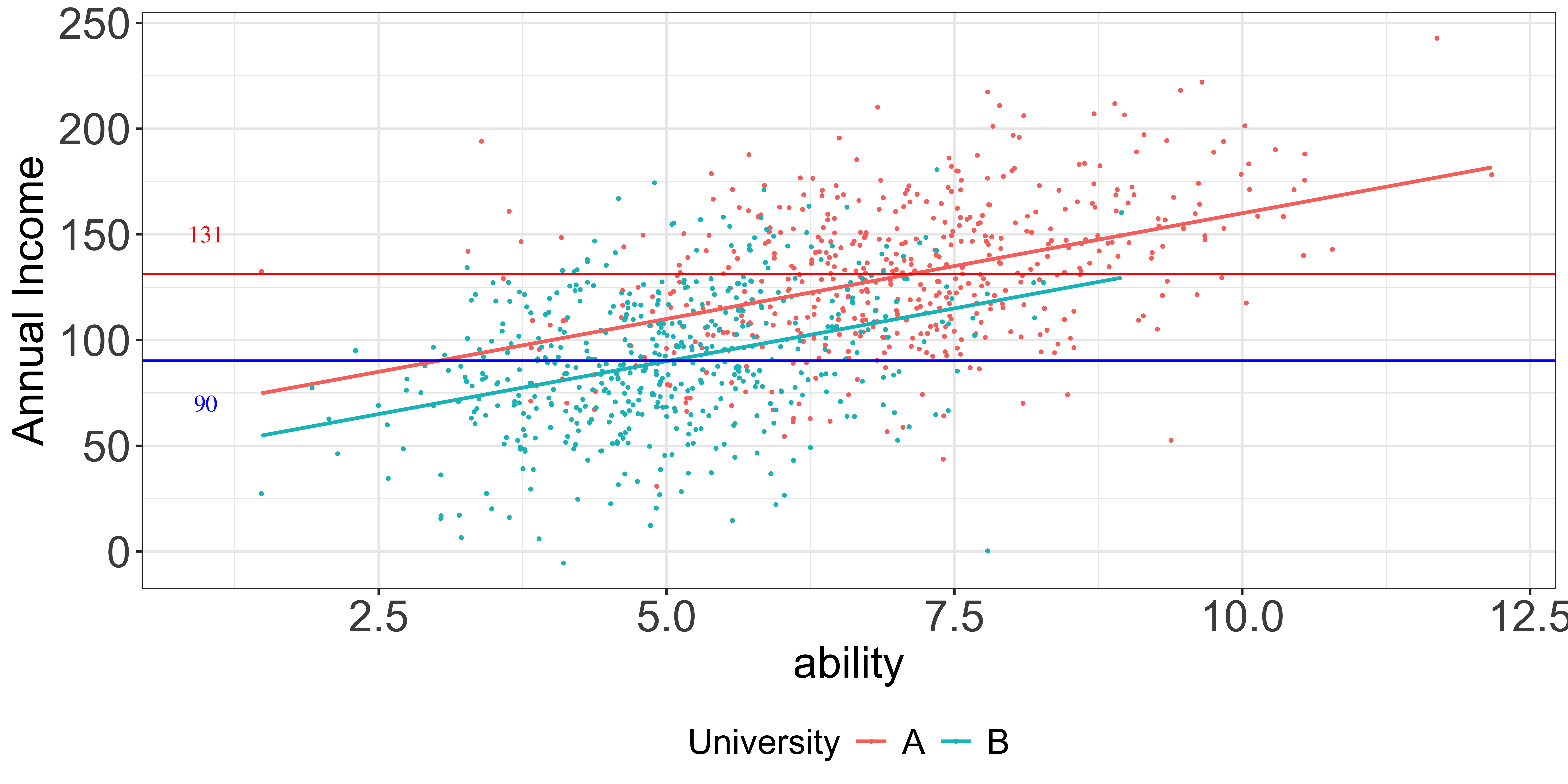
Use the figure to answer the zero conditional mean question with your eyes. Each point is a graduate, the horizontal axis is ability, and the vertical axis is annual income. Red identifies University A and blue identifies University B. The scatter around each sloped line reflects the random component of income beyond the systematic school and ability terms.

The two horizontal lines are the sample mean incomes for the universities. As the callout says, their vertical gap is about 40.9, the raw difference from the table. If you regress income only on the College A indicator, the estimated coefficient is exactly this difference in sample means. That is what the available one-variable model would report.

The sloped lines hold ability in view. At any chosen position on the ability axis, the red conditional-income line for A is twenty units above the blue line for B. Their common positive slope means that one additional ability point is associated with ten additional income units within either university. The twenty-unit vertical separation is the school effect for otherwise equally able people.

The two gaps differ because the groups occupy different parts of the horizontal axis. The red A cloud is centered farther right, around ability seven, while the blue B cloud is centered around five. Higher-ability students are more likely to be admitted to or choose A, and ability also predicts greater income. Because ability is omitted from the displayed regression model, it sits in u. Its conditional average is higher for College A equal to one than for College A equal to zero, so expected u given College A is not zero.

The zero conditional mean condition therefore fails. The raw beta-one estimate combines roughly twenty units of school effect with roughly twenty additional units due to ability differences. That is omitted-variable confounding. Flip to the final tab to see the same model when the two schools receive comparable students.
Note

The horizontal lines are the two group averages: their gap is the 40.9 from the table. The sloped lines are the two groups at a given ability: their gap is 20.

Transcript

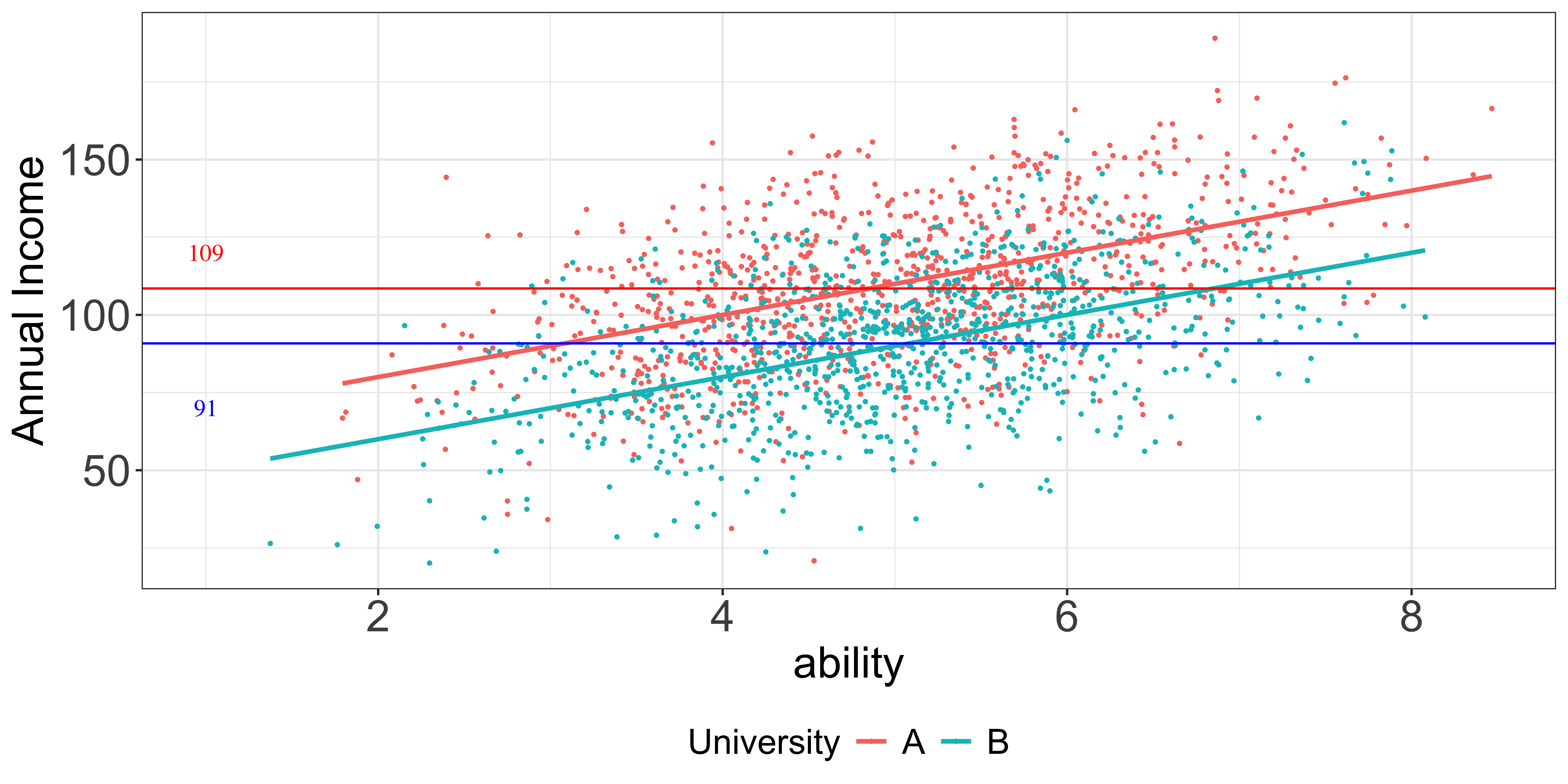
This is the counterfactual world in which college choice and ability are unrelated. The axes and colors are the same as on the previous figure: ability is on the horizontal axis, annual income is on the vertical axis, red is University A, and blue is University B. Each school again has one thousand simulated students in this version.

First inspect the point clouds along the horizontal axis. They now cover essentially the same ability range and have nearly the same center. In the realized data, mean ability is about 4.98 at A and 5.02 at B. Unlike the earlier figure, the A students are not systematically shifted toward higher ability. The two sloped lines are still parallel and twenty income units apart, because the causal school effect built into the data remains twenty at every fixed ability.

Now inspect the horizontal group-mean lines. Their realized separation is about 17.68, which the callout rounds to 18. That is not exactly twenty because these are finite random samples: the schools have slightly different realized average ability and different realized income shocks. “Up to sampling noise” is therefore important. Across repeated samples from this design, the raw difference is centered on the true twenty-unit effect rather than systematically inflated by ability.

Read the callout’s conclusion in terms of the error. Ability is still omitted from the one-variable college model, and individual income still contains noise. We have not suddenly observed or eliminated those factors. What changed is their relationship with the College A indicator. When both groups are drawn from the same ability distribution and assignment is unrelated to the other components of u, expected u given College A equals zero after normalization. The difference in group means then isolates the causal effect.

This is the central benefit of random assignment: it makes treated and comparison groups comparable on average, including on characteristics the researcher did not measure. Observational studies seek other credible ways to achieve the same identifying logic. The exercise asks you to diagnose that problem in a setting of your own.

This is what it would look like if college choice and ability were not correlated:
Important

Both groups now have the same ability distribution, so the gap between the group averages (18) is, up to sampling noise, the same as the 20 gap at any fixed ability. E[u|College\;A]=0 holds, and the raw difference is finally the causal effect.

Exercise

Transcript

Before the next lecture, apply the framework to a question you genuinely care about, perhaps one you might use in a paper or thesis. The first nested bullets ask you to name two variables. Choose a dependent variable, the outcome you want to explain, and an explanatory variable that you think changes or predicts that outcome. Define their units and the population clearly enough that someone else would know what one observation represents.

Next, construct the simple linear model. Say “y equals beta zero, plus beta one times x, plus u,” replacing y and x with your variables. State what beta one would mean in the units of your application: a one-unit increase in x changes y by beta one units, with everything else fixed. Also decide whether that ceteris paribus quantity is really the causal effect your research question needs.

Then identify what is in the error term. Be concrete and honest. List at least five omitted factors that actually affect y, rather than writing a vague phrase such as “other things.” If your outcome is crop yield and x is fertilizer, examples include soil quality, rainfall, seed variety, pest pressure, and farmer skill. If your outcome is wages and x is education, the list will be different.

Finally, take each omitted factor in turn and ask whether it is systematically related to x. Give a reason and, when possible, a likely direction. Do people choose x in response to that factor? Does an institution assign x using it? Could the factor cause both x and y? Remember that expected u equals zero overall is not the test. The relevant question is whether the combined error has mean zero at every value of x.

If one or more important determinants of y are correlated with x, a raw univariate regression will generally not identify the ceteris paribus causal effect. That is not a failed topic. It is an early diagnosis of the design problem your project must solve, using controls, an experiment, a natural experiment, panel methods, or another strategy introduced later in the course. Bring the model and your list so we can discuss which comparisons would make beta one credible.

  • consider a phenomenon you are interested in understanding
    • dependent variable (variable to be explained)
    • explanatory variable (variable to explain)
  • construct a simple linear model
  • identify what is in the error term
  • check if they are correlated with the explanatory variable or not